Article

• 1: Adopting the Victoria observability stack in Pigsty
• 2: PGCon.Dev 2024: The Week PostgreSQL Commits Paused
• 3: PostgreSQL Macro Query Optimization with pg_stat_statements
• 4: Monitor Existing PostgreSQL with Pigsty: RDS, PolarDB, and Self-Hosted Databases
• 5: Diagnose PostgreSQL slow queries
• 6: The First Pigsty Release
• 7: Golden Monitoring Metrics: Errors, Latency, Throughput, Saturation
• 8: Introducing Pigsty, a PostgreSQL Monitoring System
• 9: PostgreSQL's KPI
• 10: An Overview of PostgreSQL Monitoring
• 11: Relation Bloat Monitoring and Management
• 12: Monitoring Table Size in PostgreSQL
• 13: PostgreSQL Server Log Configuration

1 - Adopting the Victoria observability stack in Pigsty

This article describes the Pigsty v4 beta in December 2025.

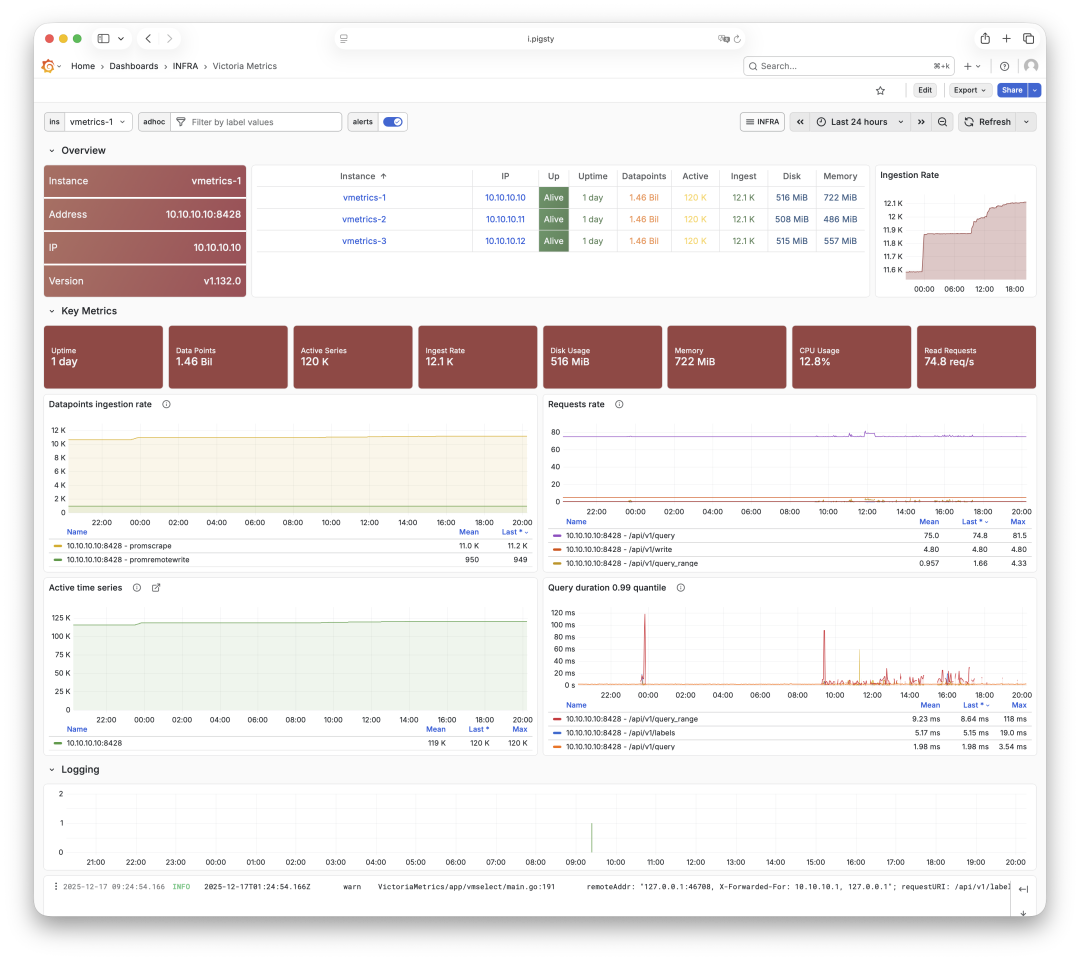
While preparing Pigsty v4.0, I replaced the default Prometheus and Loki services with VictoriaMetrics and VictoriaLogs. I also added VictoriaTraces. The aim was to reduce storage and memory use and improve dashboard and log-query response time.

Previous experience

At Tantan, we monitored about 50 million time series with twelve Prometheus nodes, each with 64 CPU cores and 256 GB of memory. In my tests, a three-node VictoriaMetrics cluster handled the workload; a larger single server also handled it. Memory and disk use were roughly one quarter of the previous setup, and queries were about four times faster.

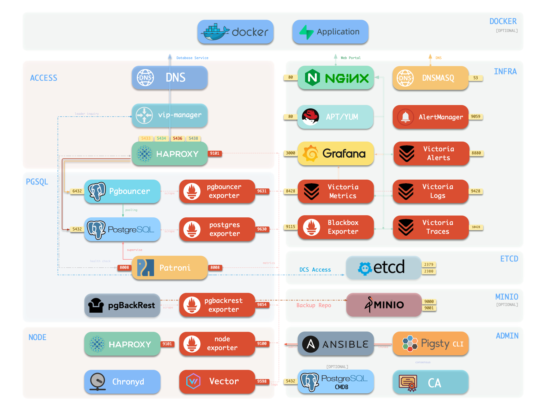
Pigsty initially offered VictoriaMetrics as an optional module. A deployment for the video production team Media Storm (影视飓风), together with the planned retirement of Promtail, prompted the infrastructure update. Promtail was the log collection agent; Loki itself was not being retired.

Aliaksandr Valialkin’s work on allocation control and efficient storage also prompted me to test the system.

Ten-node test

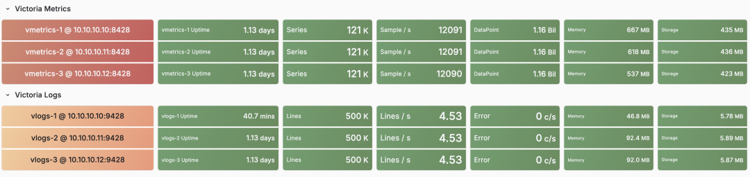
For the v4 beta, I collected metrics and logs from ten nodes. After one day, the test showed:

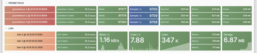
I also ran the Pigsty v3.7 Prometheus and Loki setup on ten nodes. After ten hours, its resource use was near or above the Victoria setup. The readings cover different collection periods: ten hours for Prometheus and Loki, and one day for Victoria.

The practical improvement was faster dashboard loading and log searches in this environment.

Metrics, logs, and traces

VictoriaMetrics accepts Prometheus metrics and provides a compatible query API. PG Exporter continues to expose the same /metrics endpoint. Existing dashboards can use VictoriaMetrics as their data source; check query results when migrating because MetricsQL has differences from PromQL. Recording and alert rules are evaluated by the separate vmalert service.

VictoriaMetrics supports both single-server and cluster deployments.

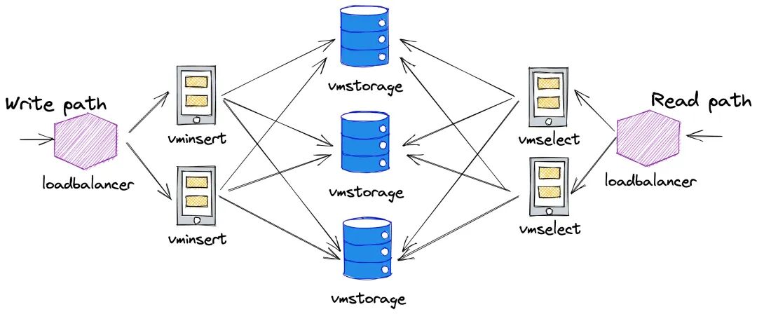
For this workload, one server had enough capacity. I used independent single-server replicas to provide redundancy without managing distributed storage. Each replica collected and stored the metrics separately.

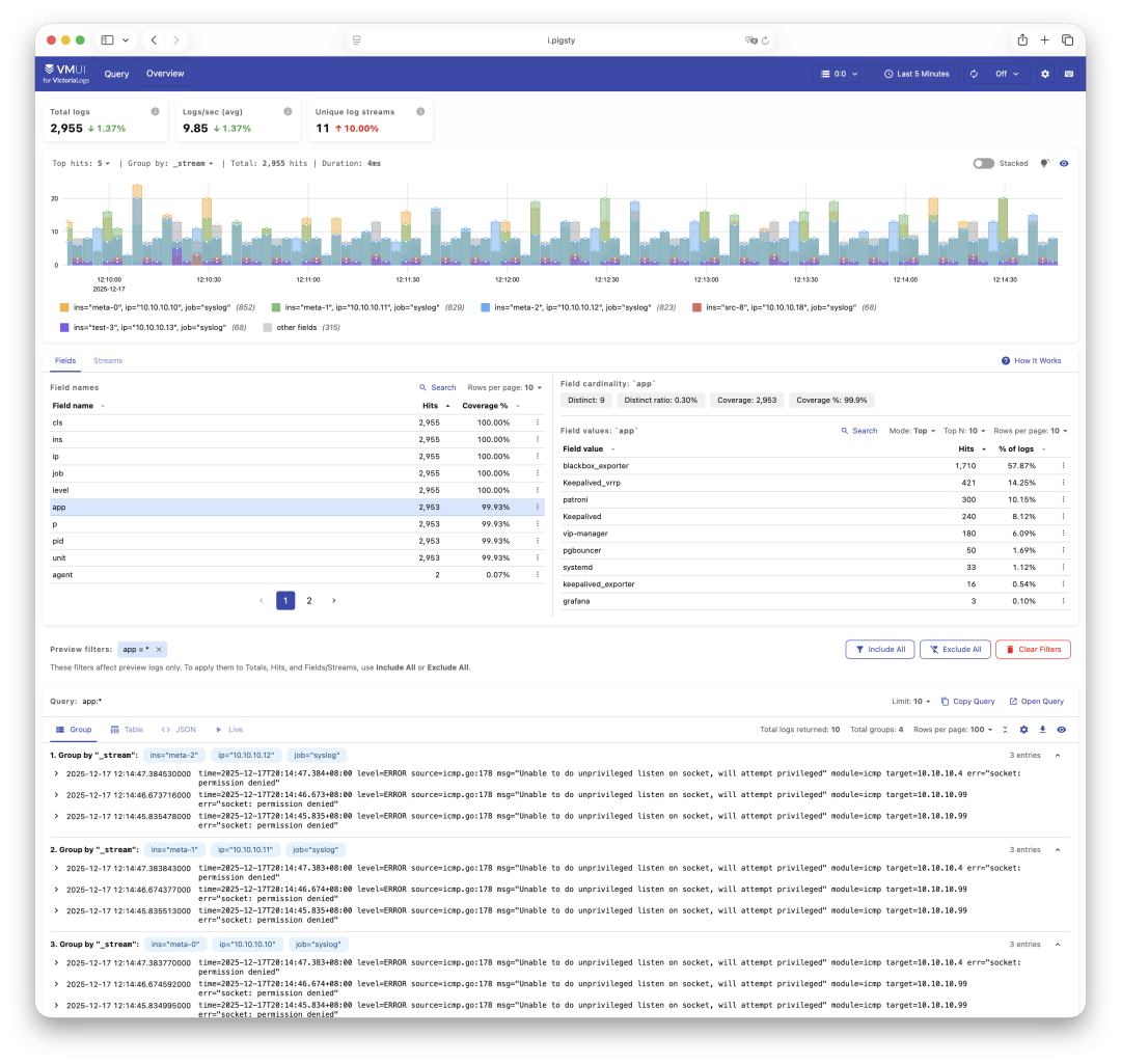
In the previous setup, expanding the log search interval could make Loki queries time out. Faster log searches were a main reason for adopting VictoriaLogs.

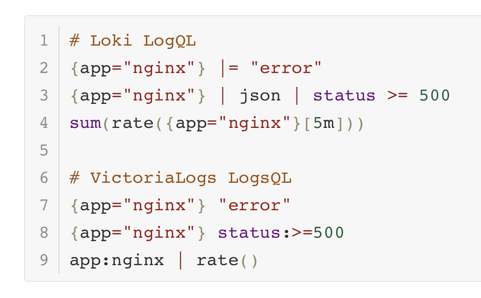
VictoriaLogs stores logs and uses LogsQL. Moving from Loki requires changing LogQL queries and the log collection configuration. In this deployment, Vector replaced Promtail.

LogsQL allows a search without a stream selector. For example, "error" "timeout" searches for log entries containing both terms. This is useful when the affected service is not yet known. See the VictoriaLogs documentation.

VictoriaTraces supplies trace storage. This beta test covered metrics and logs.

Pigsty integration

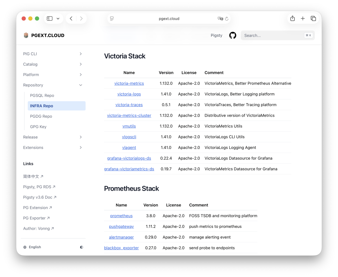
The Pigsty infrastructure repository provides RPM and DEB packages for Victoria components, tools, and Grafana plugins. The infra deployment configures storage directories, services, Grafana data sources, dashboards, and Nginx routes.

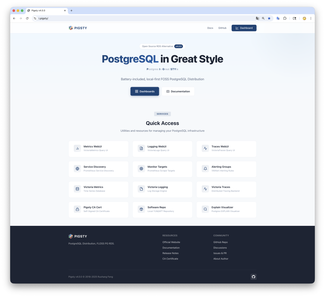
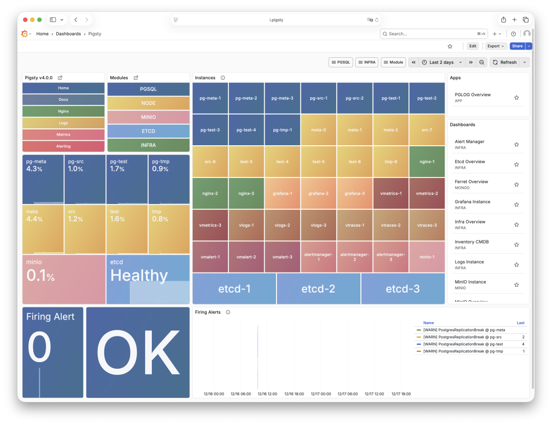
Nginx exposes the services through the configured infrastructure domain. The stack includes VictoriaMetrics, VictoriaLogs, VictoriaTraces, Grafana, vmalert, and Alertmanager.

The deployment also configures service monitoring. Additional application targets can be added through scrape configuration.

The beta deployment

The December 2025 beta used the infra configuration template to install monitoring services without PostgreSQL or etcd. The commands below show that workflow. For a new host, use the current Pigsty infrastructure guide.

curl -fsSL https://repo.pigsty.cc/beta | bash
cd ~/pigsty
./configure -c infra
./infra.yml

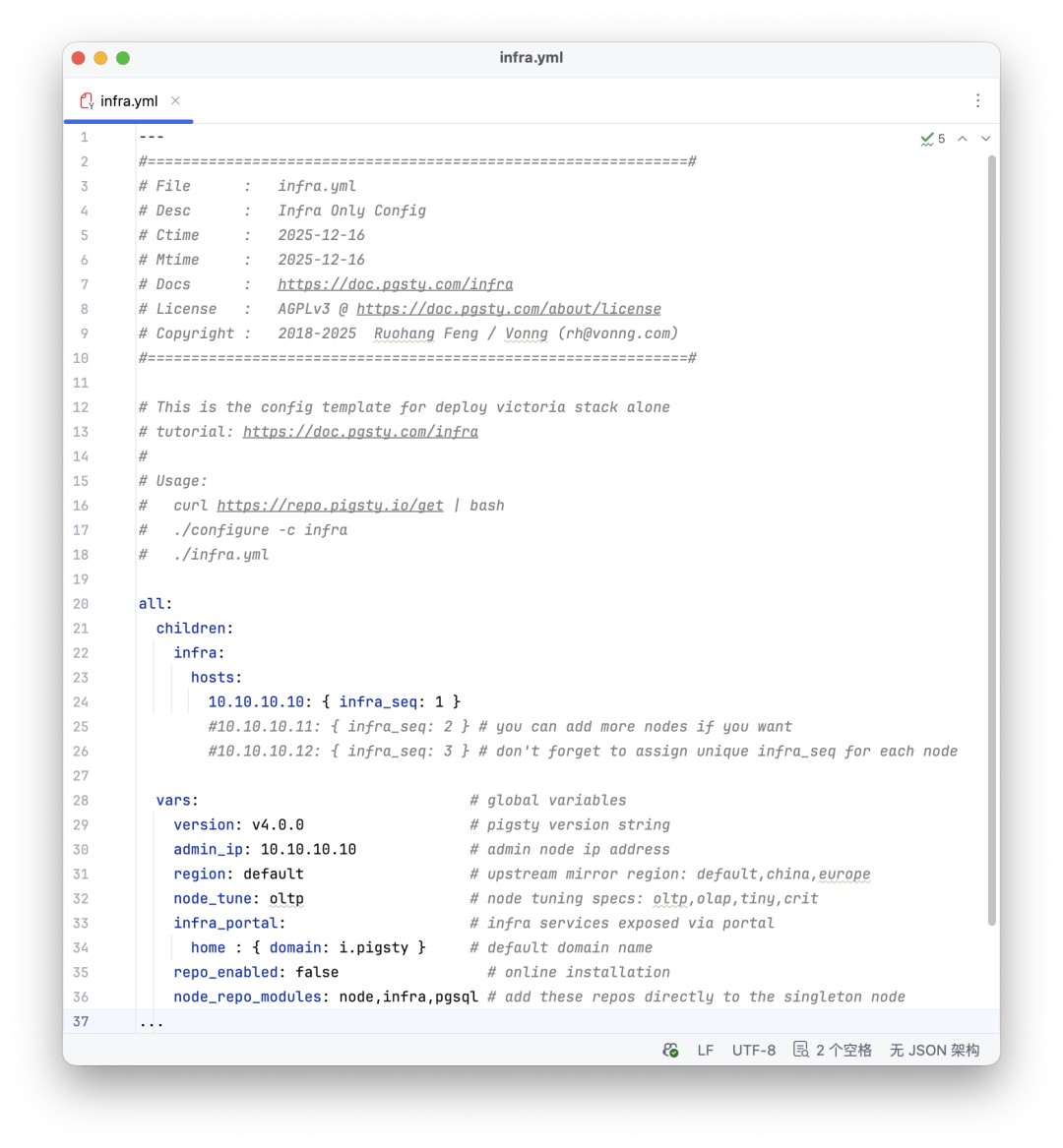
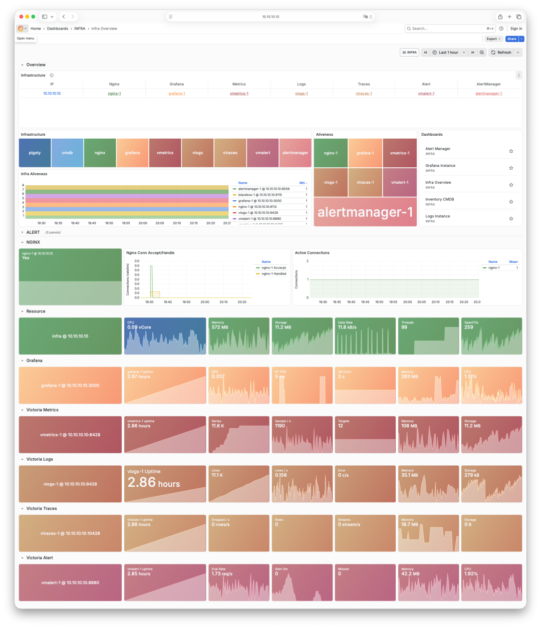
With three infrastructure nodes, the template deployed three independent replicas.

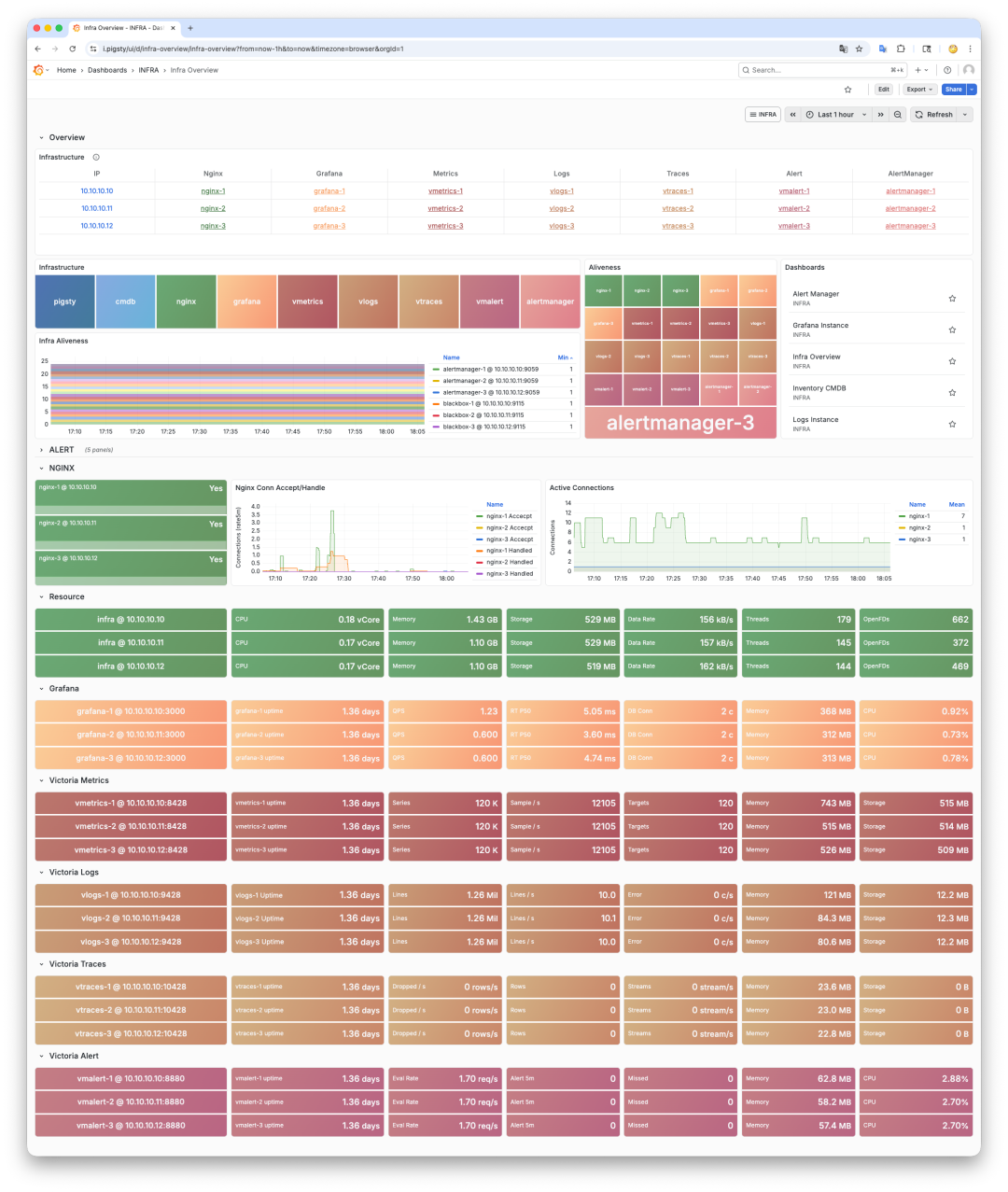
At the time of writing, the remaining v4.0 work included dashboards and documentation, with a stable release planned for January 2026. Native distributed Victoria deployment was a later task.

This migration gave me a monitoring stack that used fewer resources and responded faster under our workload. Those were the reasons to make it the Pigsty default.

2 - PGCon.Dev 2024: The Week PostgreSQL Commits Paused

This is a June 2024 conference report. Roles, package counts, and proposals reflect that event.

PGCon, the predecessor to PGCon.Dev, was held in Ottawa from 2007 through 2023. It brought PostgreSQL developers together to discuss the project’s direction.

In 2024, a new organizing team took over from Dan Langille and moved the event to SFU’s Harbour Centre in Vancouver.

Peter Eisentraut found a gap of six days, twelve hours, and forty-nine minutes between PostgreSQL commits around the conference. It was the longest gap in more than twenty years. The developers had plenty to discuss in person.

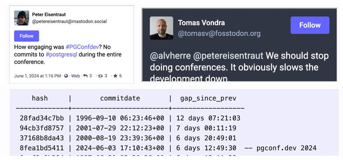
The three longer gaps all occurred early in the project’s history.

I’ve been embracing PostgreSQL for a decade, but attending a global PG Hacker conference in person was a first for me, and I’m immensely grateful for the organizer’s efforts. PGCon.Dev 2024 wrapped up on May 31st, though this post comes a bit delayed as I’ve been exploring Vancouver and Banff National Park ;)

Day Zero: Extension Summit

Day zero was for leadership meetings, and I signed up for the afternoon’s Extension Ecosystem Summit.

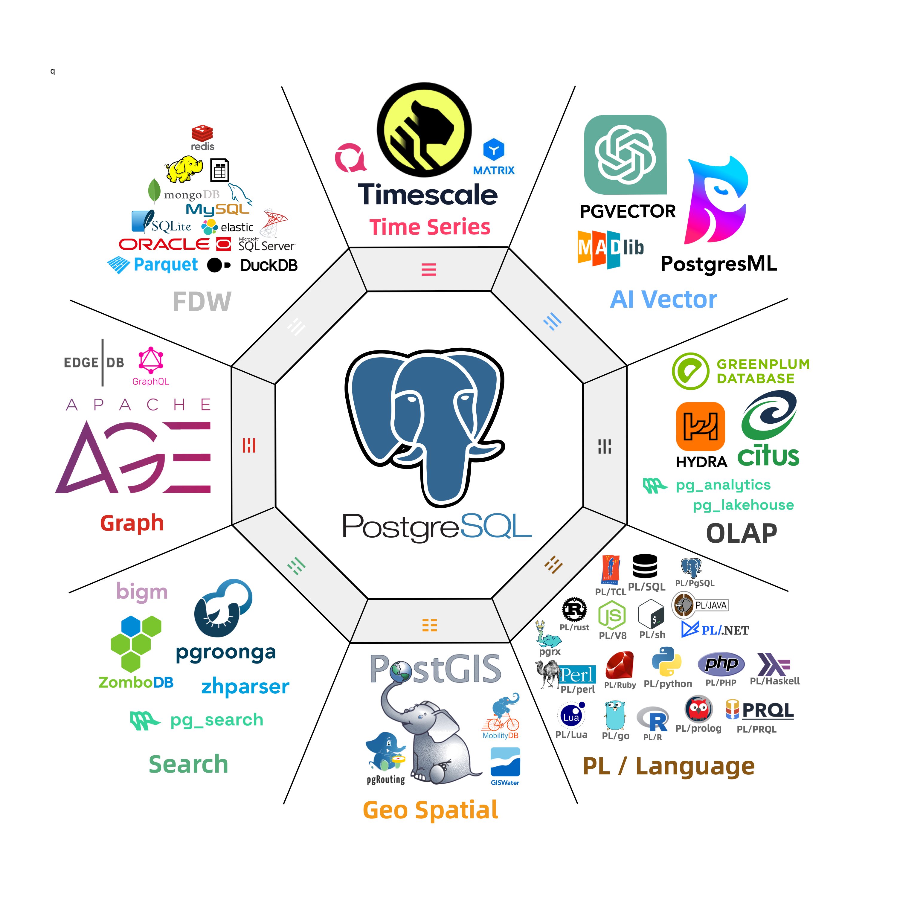
Maybe this summit is somewhat subtly related to my recent post, “Postgres is eating the database world,” highlighting PostgreSQL’s thriving extension ecosystem as a unique and critical success factor and drawing the community’s attention.

I joined David Wheeler’s Binary Packaging session with the RPM and APT maintainers. They questioned the need for new distribution standards such as PGXN v2. In the second half, I attended Yurii Rashkovskii’s discussion of extension directories, metadata, naming conflicts, versioning, and binary distribution.

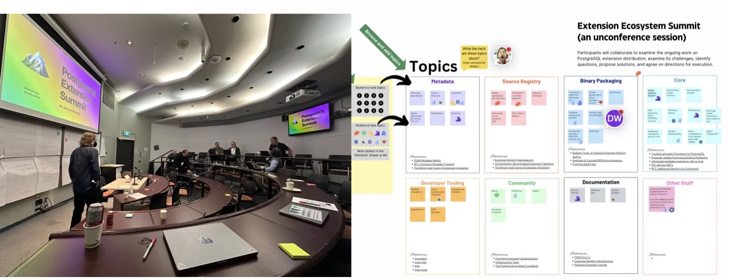
Prior to this summit, the PostgreSQL community had held six mini-summits discussing these topics intensely, with visions for the extension ecosystem’s future development shared by various speakers. Recordings of these sessions are available on YouTube.

And after the summit, I had a chance to chat with Devrim, the RPM maintainer, about extension packaging, which was quite enlightening.

“Keith Fan Group” – from Devrim on Extension Summit

Day One: Brilliant Talks and Bar Social

The core of PGCon.Dev lies in its sessions. Unlike some China domestic conferences with mundane product pitches or irrelevant tech details, PGCon.Dev presentations are genuinely engaging and substantive. The official program kicked off on May 29th, after a day of closed-door leadership meetings and the Ecosystem Summit on the 28th.

The opening was co-hosted by Jonathan Katz, 1 of the 7 core PostgreSQL team members and a chief product manager at AWS RDS, and Melanie Plageman, a recent PG committer from Microsoft. A highlight was when Andres Freund, the developer who uncovered the famous xz backdoor, was celebrated as a superhero on stage.

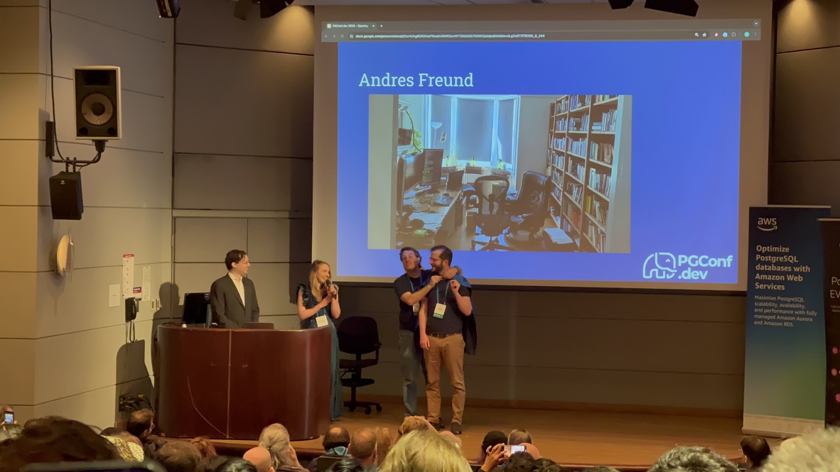
Following the opening, the regular session tracks began. Although conference videos aren’t out yet, I’m confident they’ll “soon” be available on YouTube. Most sessions had three tracks running simultaneously; here are some highlights I chose to attend.

Pushing the Boundaries of PG Extensions

Yurii’s talk, “Pushing the Boundaries of PG Extensions,” tackled what kind of extension APIs PostgreSQL should offer. PostgreSQL boasts robust extensibility, but the current extension API set is decades old, from the 9.x era. Yurii’s proposal aims to address issues with the existing extension mechanisms. Challenges such as installing multiple versions of an extension simultaneously, avoiding database restarts post-extension installations, managing extensions as seamlessly as data, and handling dependencies among extensions were discussed.

Yurii and Viggy, founders of Omnigres, aim to transform PostgreSQL into a full-fledged application development platform, including hosting HTTP servers directly within the database. They designed a new extension API and management system for PostgreSQL to achieve this. Their innovative improvements represent the forefront of exploration into PostgreSQL’s core extension mechanisms.

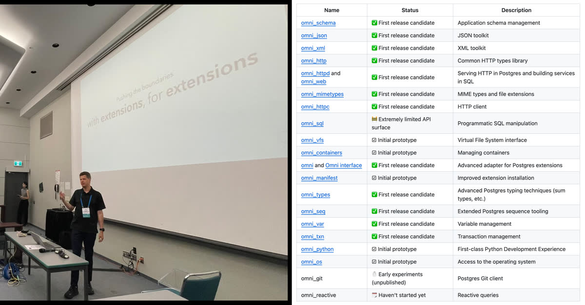
I had a great conversation with Viggy and Yurii. Yurii walked me through compiling and installing Omni. I plan to support the Omni extension series in the next version of Pigsty, making this powerful application development framework plug-and-play.

Anarchy in DBMS

Abigale Kim from CMU, under the mentorship of celebrity professor Andy Pavlo, delivered the talk “Anarchy in the Database—A Survey and Evaluation of DBMS Extensibility.” This topic intrigued me since Pigsty’s primary value proposition is about PostgreSQL’s extensibility.

In Kim’s comparison, PostgreSQL supported nine of the ten extension points studied, the broadest coverage among the surveyed systems. Her survey listed more than 375 PostgreSQL extensions.

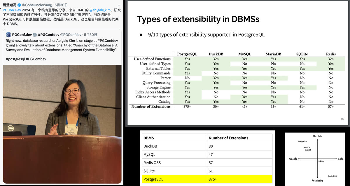
Kim’s quantitative analysis of compatibility levels among these extensions resulted in a compatibility matrix, unveiling conflicts—most notably, powerful extensions like TimescaleDB and Citus are prone to clashes. This information is very valuable for users and distribution maintainers. Read the detailed study.

I told Kim that her research provided concrete data for comparing database extensibility.

How PostgreSQL is Misused and Abused

Karen Jex from Crunchy Data brought a user’s perspective to the first afternoon session. She described mistakes commonly made by PostgreSQL beginners. The examples were familiar to me, but useful for developers who rarely see how newcomers use the database.

PostgreSQL and the AI Ecosystem

The second-afternoon session by Bruce Momjian, co-founder of the PGDG and a core committee member from the start, was unexpectedly about using PostgreSQL’s multi-dimensional arrays and queries to implement neural network inference and training.

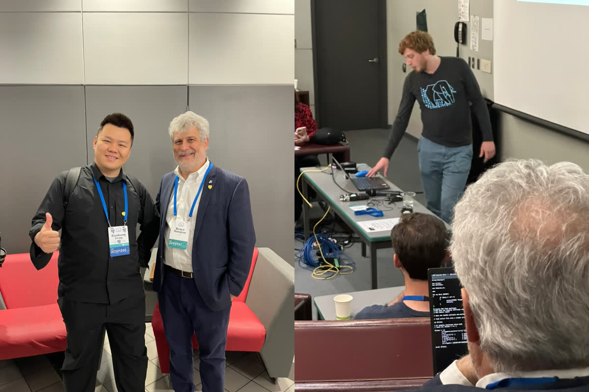
Haha, some ArgParser code. I see it

During the lunch, Bruce explained that Jonathan Katz needed a topic to introduce the vector database extension PGVector in the PostgreSQL ecosystem, so Bruce was roped in to “fill the gap.”

PB-Level PostgreSQL Deployments

Chris Travers reported moving a workload from Elasticsearch to a partitioned and sharded PostgreSQL deployment. The earlier system retained 1 PB for 30 days; the PostgreSQL deployment described in his slides stored 10 PB. I found the operating experience at that scale particularly interesting.

Highlight: When Hardware and Database Collide

My favorite talk at this conference was Margo Seltzer’s “When Hardware and Database Collide”.

Margo Seltzer is a professor at UBC, formerly at Harvard, a member of the National Academy of Engineering, and one of the authors of BerkeleyDB. She discussed challenges facing databases today. She pinpointed that the bottleneck for databases has shifted from disk I/O to main memory speed. Emerging hardware technologies like HBM and CXL could be the solution, posing new challenges for PostgreSQL hackers to tackle.

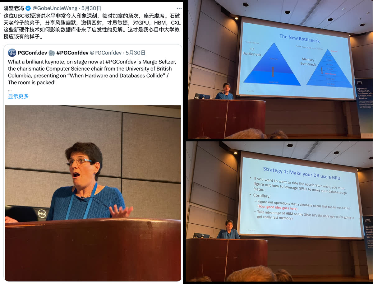
I enjoyed Margo’s direct and engaging presentation. I would like to watch it again when the conference video is available.

WetBar Social

Following Margo’s session, the official Social Event took place at Rogue Kitchen & Wetbar, just a street away from the venue at Waterfront Station, boasting views of the Pacific and iconic Vancouver landmarks.

The informal setting was perfect for engaging with new and old peers. Conversations with notable figures like Devrim, Tomasz, Yurii, and Keith were particularly enriching. As an RPM maintainer, I had an extensive and fruitful discussion with Devrim, resolving many longstanding queries.

The atmosphere was warm and familiar, with many reconnecting after long periods. A couple of beers in, conversations flowed even more freely among fellow PostgreSQL enthusiasts. The event concluded with an invitation from Melanie for a board game session, which I regretfully declined due to my limited English in such interactive settings.

Day 2: Debate, Lunch, and Lightning Talks

Multi-Threading Postgres

The warmth from the previous night’s socializing carried over into the next day, marked by the eagerly anticipated session on “Multi-threaded PostgreSQL,” which was packed to capacity. The discussion, initiated by Heikki, centered on the pros and cons of PostgreSQL’s process and threading models, along with detailed implementation plans and current progress.

Heikki described potential benefits of a threading model: cheaper connections, shared relation and plan caches, adjustable shared memory, and easier memory limits. The discussion also covered isolation, bugs, and compatibility changes that extension authors would need to handle.

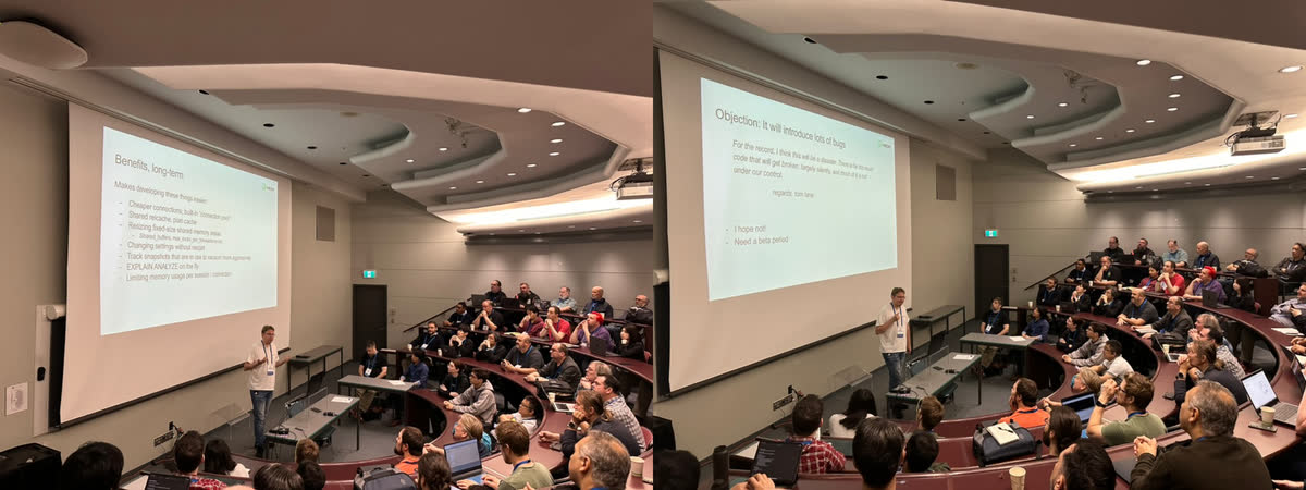
Heikki laid out a detailed plan to transition to the threading model over five to seven years, aiming for a seamless shift without intermediate states. Intriguingly, he cited Tom Lane’s critical comment in his presentation:

For the record, I think this will be a disaster. There is far too much code that will get broken, largely silently, and much of it is not under our control. – regards, tom lane

Although Tom Lane smiled benignly without voicing any objections, the strongest dissent at the conference came not from him but from an extension maintainer. The elder developer, who maintained several extensions, raised concerns about compatibility, specifically regarding memory allocation and usage. Heikki suggested that extension authors should adapt their work to a new model during a transition grace period of about five years. This suggestion visibly upset the maintainer, who left the meeting in anger.

Given the proposed threading model’s significant impact on the existing extension ecosystem, I’m skeptical about this change. At the conference, I consulted on the threading model with Heikki, Tom Lane, and other hackers. The community’s overall stance is one of curious & cautious observation. So far, the only progress is in PG 17, where the fork-exec-related code has been refactored and global variables marked for future modifications. Any real implementation would likely not occur until at least PG 20+.

Hallway Track

The sessions on the second day were slightly less intense than the first, so many attendees chose the “Hallway Track”—engaging in conversations in the corridors and lobby. I’m usually not great at networking as an introvert, but the vibrant atmosphere quickly drew me in. Eye contact alone was enough to spark conversations, like triggering NPC dialogue in an RPG. I also managed to subtly promote Pigsty to every corner of the PG community.

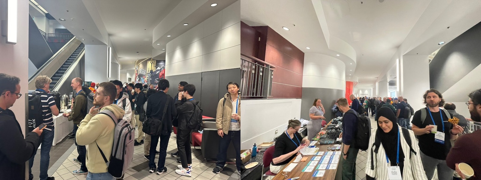
Despite being a first-timer at PGCon.Dev, I was surprised by the recognition and attention I received, largely thanks to the widely read article, “PostgreSQL is eating the Database world.” Many recognized me by my badge Vonng / Pigsty.

A simple yet effective networking trick is never to underestimate small gifts’ effect. I handed out gold-plated Slonik pins, PostgreSQL’s mascot, which became a coveted item at the conference. Everyone who talked with me received one, and those who didn’t have one were left asking where to get one. LOL

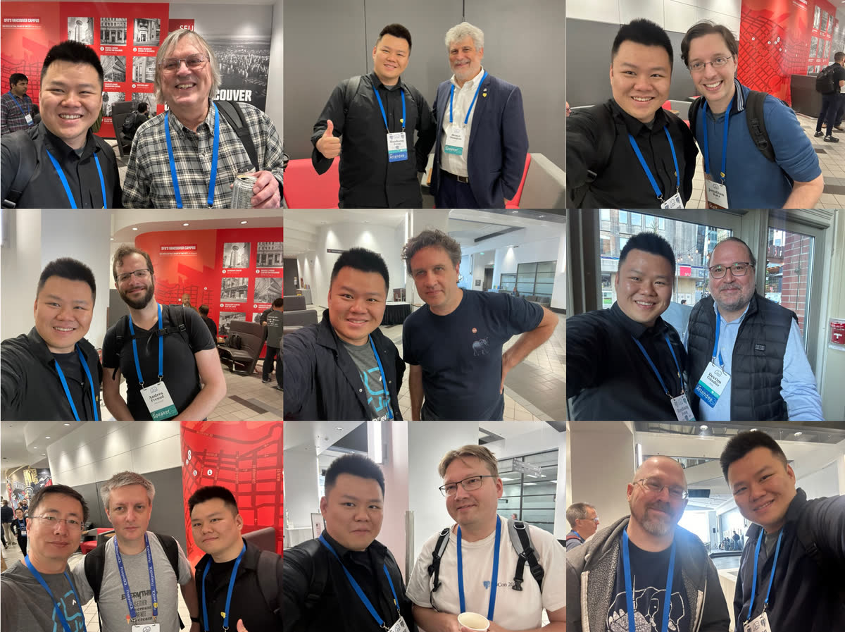
Anyway, I’m glad to have made many new friends and connections.

Multinational Community Lunch

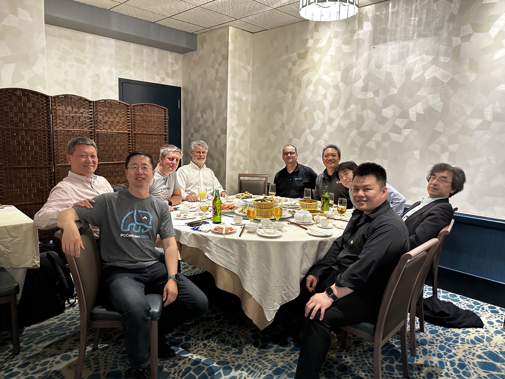
As for lunch, HighGo hosted key participants from the American, European, Japanese, and Chinese PostgreSQL communities at a Cantonese restaurant in Vancouver. The conversation ranged from serious technical discussions to lighter topics. I met Tatsuro Yamada, who gave the talk “Advice is seldom welcome but efficacious”, and Kyotaro Horiguchi, a core contributor to PostgreSQL known for his work on WAL replication and multibyte string processing and the author of pg_hint_plan.

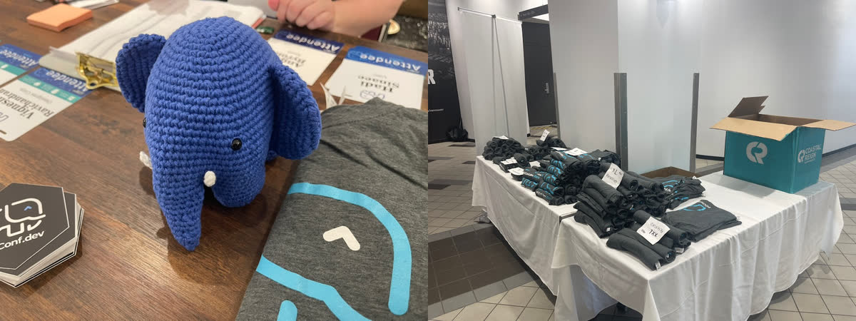
Another major contributor to the PostgreSQL community, Mark Wong organizes PGUS and has developed a series of PostgreSQL monitoring extensions. He also manages community merchandise like contributor coins, shirts, and stickers. He even handcrafted a charming yarn elephant mascot, which was so beloved that one was sneakily “borrowed” at the last PG Conf US.

Bruce, already a familiar face in the PG Chinese community, Andreas Scherbaum from Germany, organizer of the European PG conferences, and Miao Jian, founder of Han Gao, representing the only Chinese database company at PGCon.Dev, all shared insightful stories and discussions about the challenges and nuances of developing databases in their respective regions.

On returning to the conference venue, I had a conversation with Jan Wieck, a former PostgreSQL core team member. He shared his story of participating in the PostgreSQL project from the early days and encouraged me to get more involved in the PostgreSQL community, reminding me its future depends on the younger generation.

Making PG Hacking More Inclusive

At PGCon.Dev, a special session on community building chaired by Robert Haas, featured three new PostgreSQL contributors sharing their journey and challenges, notably the barriers for non-native English speakers, timezone differences, and emotionally charged email communications.

Robert emphasized in a post-conference blog his desire to see more developers from India and Japan rise to senior positions within PostgreSQL’s ranks, noting the underrepresentation from these countries despite their significant developer communities.

While we’re at it, I’d really like to see more people from India and Japan in senior positions within the project. We have very large developer communities from both countries, but there is no one from either of those countries on the core team, and they’re also underrepresented in other senior positions. At the risk of picking specific examples to illustrate a general point, there is no one from either country on the infrastructure team or the code of conduct committee. We do have a few committers from those countries, which is very good, and I was pleased to see Amit Kapila on the 2024.pgconf.dev organizing commitee, but, overall, I think we are still not where we should be. Part of getting people involved is making them feel like they are not alone, and part of it is also making them feel like progression is possible. Let’s try harder to do that.

The discussion mentioned India and Japan but not China, which left me with mixed feelings. I would like to see more sustained upstream participation from Chinese users and developers. Richard Guo from PieCloudDB had become a PostgreSQL committer that year.

As far as I knew, five attendees had come from China: four from HighGo and me.

I hope my participation helps more users and developers in the Chinese-speaking community make connections, share their work with the global community, and find opportunities to collaborate.

Lightning Talks

The second day ended with lightning talks, each limited to five minutes. Eleven speakers covered their topics in 45 minutes. Keith discussed PG Monitor improvements, and Peter Eisentraut covered SQL standard updates. My highlight was Devrim Gündüz’s talk on PG RPMs: he fitted 75 slides into five minutes, delivering the “big reveal” he had promised at the bar.

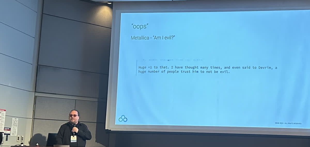
Many PostgreSQL users install binary packages rather than build from source. At the time, I maintained packages for 34 extensions in Pigsty, while Devrim maintained more than a hundred in the PGDG RPM repository. This packaging work makes extensions available to a much wider audience.

Devrim is a fascinating character — a Turkish native living in London, a part-time DJ, and the maintainer of the PGDG RPM repository, sporting a PostgreSQL logo tattoo. After an engaging chat about the PGDG repository, he shared insights on how extensions are added, highlighting the community-driven nature of PGXN and recent popular additions like pgvector, (which I made the suggestion haha).

Interestingly, with the latest Pigsty v2.7 release, four of my maintained (packaging) extensions (pgsql-http, pgsql-gzip, pg_net, pg_bigm) were adopted into the PGDG official repository. Devrim admitted to scouring Pigsty’s extension list for good picks, though he humorously dismissed any hopes for my Rust pgrx extensions making the cut, reaffirming his commitment to not blending Go and Rust plugins into the official repository. Our conversation was so enriching that I’ve committed myself to becoming a “PG Extension Hunter,” scouting and recommending new plugins for official inclusion.

Day 3: Unconference

One of the highlights of PGCon.Dev is the Unconference, a self-organized meeting with no predefined agenda, driven by attendee-proposed topics. On day three, Joseph Conway facilitated the session where anyone could pitch topics for discussion, which were then voted on by participants. My proposal for a Built-in Prometheus Metrics Exporter was merged into a broader Observability topic spearheaded by Jeremy.

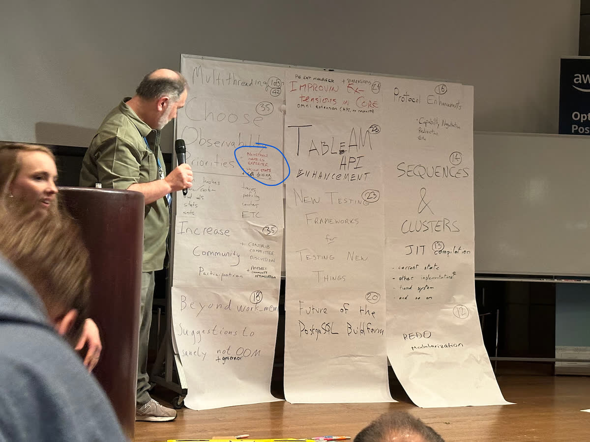
The top-voted topics were Multithreading (42 votes), Observability (35 votes), and Enhanced Community Engagement (35 votes). Observability features were a major focus, reflecting the community’s priority. I proposed integrating a contrib monitoring extension in PostgreSQL to directly expose metrics via HTTP endpoint, using pg_exporter as a blueprint but embedded to overcome the limitations of external components, especially during crash recovery scenarios.

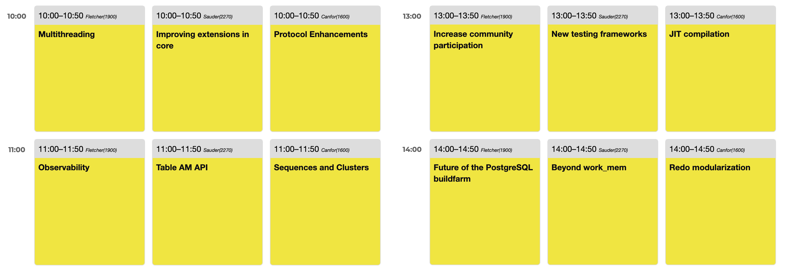
There’s a clear focus on observability among the community. As the author of pg_exporter, I proposed developing a first-party monitoring extension. This extension would integrate Prometheus monitoring endpoints directly into PostgreSQL, exposing metrics via HTTP without needing external components.

The proposal aimed to reduce the need to manage a separate exporter and expose internal state while SQL connections were unavailable, such as during crash recovery. Those capabilities would require implementation and testing in PostgreSQL.

The suggested implementation involves a background worker process similar to the bgw_replstatus extension. This process would listen on an additional port to expose monitoring metrics through HTTP, using pg_exporter as a blueprint. Metrics would primarily be defined via a Collector configuration table, except for a few critical system indicators.

This idea garnered attention from several PostgreSQL hackers at the event. Developers from EDB and CloudNativePG are evaluating whether pg_exporter could be directly integrated into their distributions as part of their monitoring solutions. And finally, an Observability Special Interest Group (SIG) was formed by attendees interested in observability, planning to continue discussions through a mailing list.

Issue: Support for LoongArch Architecture

During the last two days, I have had some discussions with PG Hackers about some Chinese-specific issues.

One suggestion was to add LoongArch builds to the PGDG repositories, with build infrastructure offered by Chinese chip and operating-system vendors. Devrim said the RPM build distributions did not support the architecture at that time. Tomasz Rybak was open to Debian packages if the architecture became available in Debian 13.

In summary, official PG RPMs might not yet support LoongArch, but APT has a chance, contingent on broader OS support for mainstream open-source Linux distributions.

Issue: Server-side Chinese Character Encoding

Jeremy Schneider’s talk on collation described problems caused by changes in sorting rules. His preference for simple, stable ordering matched my own practice. His slides explain the tradeoffs.

After the talk, Jeremy, Peter Eisentraut, and I discussed GB18030 compatibility. PostgreSQL supported this encoding for clients and conversion functions, but not as a server encoding. I also raised a possible mapping problem affecting about twenty added Chinese characters in convert_to(..., 'gb18030'). They agreed to investigate.

Closing

The event closed with Jonathan Katz and Melanie Plageman wrapping up an exceptional conference that leaves us looking forward to next year’s PGCon.Dev 2025 in Canada, possibly in Vancouver, Toronto, Ottawa, or Montreal.

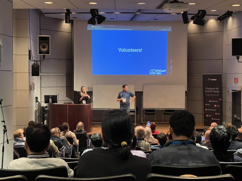
Inspired by the engagement at this conference, I’m considering presenting on Pigsty or PostgreSQL observability next year.

Notably, following the conference, Pigsty’s international CDN traffic spiked significantly, highlighting the growing global reach of our PostgreSQL distribution, which really made my day.

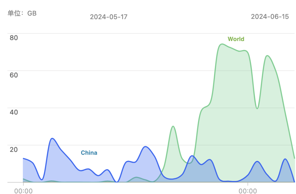
Pigsty CDN Traffic Growth after PGCon.Dev 2024

The official session archive contains slides. Other reports include:

• Andreas Scherbaum PostgreSQL Development Conference 2024 - Review

• PgCon 2024 Developer Meeting

• Robert Haas: 2024.pgconf.dev and Growing the Community

• How engaging was PGConf.dev really?

• PGConf.dev 2024: Shaping the Future of PostgreSQL in Vancouver

• PGCon.Dev Extension Summit Notes @ Vancouver

• PGCon 2024 Opening

3 - PostgreSQL Macro Query Optimization with pg_stat_statements

This article describes the monitoring approach used in 2023. Its examples use PostgreSQL 15 fields and the dashboards available at that time.

Slow queries increase response times and consume database resources. They can also prolong lock contention and increase connection pressure. Query optimization is therefore a core DBA responsibility.

On the path of query optimization, there are two different approaches:

Macro Optimization: Analyze the overall workload, dissect and drill down, identifying and improving the worst-performing parts from top to bottom.

Micro Optimization: Analyze an individual query with its execution plan, slow query logs, and wait events.

Today we’ll discuss the former. Macro optimization has three main goals and motivations:

Reduce Resource Consumption: Lower the risk of resource saturation, optimize CPU/memory/IO, typically using query total time/total IO as optimization targets.

Improve User Experience: The most common optimization goal, in OLTP systems typically using reduced average query response time as the optimization target.

Balance Workload: Ensure appropriate proportional relationships in resource usage/performance between different query groups.

These goals require query-level measurements. pg_stat_statements provides them.

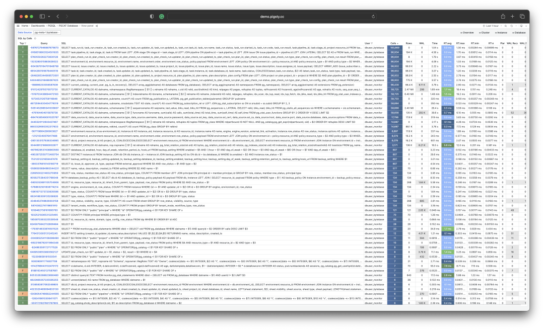
Extension: PGSS

pg_stat_statements, hereafter abbreviated as PGSS, is the core tool for practicing the macro way.

PGSS comes from the official PostgreSQL Global Development Group, distributed as a first-party extension alongside the database kernel itself, providing methods for tracking SQL statement-level metrics.

I consider PGSS essential for production monitoring. At the time of writing, Pigsty loaded it by default alongside auto_explain, which supports analysis of individual query plans.

Add pg_stat_statements to shared_preload_libraries and restart PostgreSQL. Then run CREATE EXTENSION pg_stat_statements in the database where you want to query its views. PostgreSQL 15 also needs query IDs enabled; the default compute_query_id = auto meets this requirement.

PGSS groups statements by normalized query structure, database, user, and top-level status. A group can use different execution plans. The following table definition illustrates the PostgreSQL 15 view columns; create the extension rather than executing this definition.

CREATE TABLE pg_stat_statements
(
    userid                 OID,     -- (Label) User OID executing this statement
    dbid                   OID,     -- (Label) Database OID containing this statement
    toplevel               BOOL,    -- (Label) Whether this statement is top-level SQL
    queryid                BIGINT,  -- (Label) Query ID: hash of normalized query
    query                  TEXT,    -- (Label) Normalized query statement text
    plans                  BIGINT,  -- (Counter) Number of times this statement was planned
    total_plan_time        FLOAT,   -- (Counter) Total time spent planning this statement
    min_plan_time          FLOAT,   -- (Gauge) Minimum planning time
    max_plan_time          FLOAT,   -- (Gauge) Maximum planning time
    mean_plan_time         FLOAT,   -- (Gauge) Average planning time
    stddev_plan_time       FLOAT,   -- (Gauge) Standard deviation of planning time
    calls                  BIGINT,  -- (Counter) Number of times this statement was executed
    total_exec_time        FLOAT,   -- (Counter) Total time spent executing this statement
    min_exec_time          FLOAT,   -- (Gauge) Minimum execution time
    max_exec_time          FLOAT,   -- (Gauge) Maximum execution time
    mean_exec_time         FLOAT,   -- (Gauge) Average execution time
    stddev_exec_time       FLOAT,   -- (Gauge) Standard deviation of execution time
    rows                   BIGINT,  -- (Counter) Total rows retrieved or affected by this statement
    shared_blks_hit        BIGINT,  -- (Counter) Total shared buffer blocks hit
    shared_blks_read       BIGINT,  -- (Counter) Total shared buffer blocks read
    shared_blks_dirtied    BIGINT,  -- (Counter) Total shared buffer blocks dirtied
    shared_blks_written    BIGINT,  -- (Counter) Total shared buffer blocks written to disk
    local_blks_hit         BIGINT,  -- (Counter) Total local buffer blocks hit
    local_blks_read        BIGINT,  -- (Counter) Total local buffer blocks read
    local_blks_dirtied     BIGINT,  -- (Counter) Total local buffer blocks dirtied
    local_blks_written     BIGINT,  -- (Counter) Total local buffer blocks written to disk
    temp_blks_read         BIGINT,  -- (Counter) Total temp buffer blocks read
    temp_blks_written      BIGINT,  -- (Counter) Total temp buffer blocks written to disk
    blk_read_time          FLOAT,   -- (Counter) Total time spent reading blocks
    blk_write_time         FLOAT,   -- (Counter) Total time spent writing blocks
    temp_blk_read_time     FLOAT,   -- (Counter) Total time reading temporary blocks
    temp_blk_write_time    FLOAT,   -- (Counter) Total time writing temporary blocks
    wal_records            BIGINT,  -- (Counter) Total WAL records generated
    wal_fpi                BIGINT,  -- (Counter) Total WAL full page images generated
    wal_bytes              NUMERIC, -- (Counter) Total WAL bytes generated
    jit_functions          BIGINT,  -- (Counter) Number of functions JIT-compiled
    jit_generation_time    FLOAT,   -- (Counter) Total time spent generating JIT code
    jit_inlining_count     BIGINT,  -- (Counter) Number of times functions were inlined
    jit_inlining_time      FLOAT,   -- (Counter) Total time spent inlining functions
    jit_optimization_count BIGINT,  -- (Counter) Number of times queries were JIT-optimized
    jit_optimization_time  FLOAT,   -- (Counter) Total time spent on JIT optimization
    jit_emission_count     BIGINT,  -- (Counter) Number of times code was JIT-emitted
    jit_emission_time      FLOAT,   -- (Counter) Total time spent on JIT emission
    PRIMARY KEY (userid, dbid, queryid, toplevel)
);

PostgreSQL 15 view columns. All time fields use milliseconds. The pg_query_exec_time metric used below converts execution time to seconds. I/O timing requires track_io_timing; planning statistics require pg_stat_statements.track_planning.

Execution statistics are updated when a statement finishes successfully. Use pg_stat_activity for running statements and logs for errors. If planning succeeds but execution fails, PGSS can still record the planning statistics.

queryid depends on the parsed query and referenced database objects. Physical replicas normally produce matching IDs. Do not use it as a permanent identifier across PostgreSQL major versions, logical replicas, or dropped and recreated objects.

Raw Data

Columns in the PGSS view can be divided into three categories:

Descriptive Label Columns: Query ID (queryid), database ID (dbid), user (userid), a top-level query marker, and normalized query text (query).

Measurement Metrics (Gauge): Eight statistics related to minimum, maximum, mean, and standard deviation, prefixed with min, max, mean, stddev and suffixed with plan_time and exec_time.

Cumulative Metrics (Counter): Other metrics besides the above eight columns and label columns, such as calls, rows, etc. The most important and useful metrics are in this category.

First, let’s explain queryid: queryid is a hash value generated from the normalized query after parsing the query statement and stripping constants, so it can be used to identify the same type of query. Different query statements may have the same queryid (same structure after normalization), and the same query statement may have different queryids (e.g., due to different search_path, resulting in different actual tables being queried).

The same query may be executed by different users in different databases. Therefore, in the PGSS view, the four label columns queryid, dbid, userid, toplevel together form the “primary key” that uniquely identifies a record.

For metric columns, measurement-type metrics (GAUGE) are mainly the eight statistics related to execution time and planning time, but users have no good way to control the statistical range of these statistics, so their practical value is limited.

The really important metrics are cumulative metrics (Counter), such as:

calls: How many times this query group was invoked.

total_exec_time + total_plan_time: Total time consumed by the query group.

rows: Total rows retrieved or affected by the query group.

shared_blks_hit + shared_blks_read: Total buffer pool hits and read operations.

wal_bytes: Total WAL bytes generated by queries in this group.

blk_read_time and blk_write_time: Total time spent on block read/write IO

Here, the most meaningful metrics are calls and total_exec_time, which can be used to calculate the core metrics QPS (throughput) and RT (latency/response time) for query groups, though other metrics also have reference value.

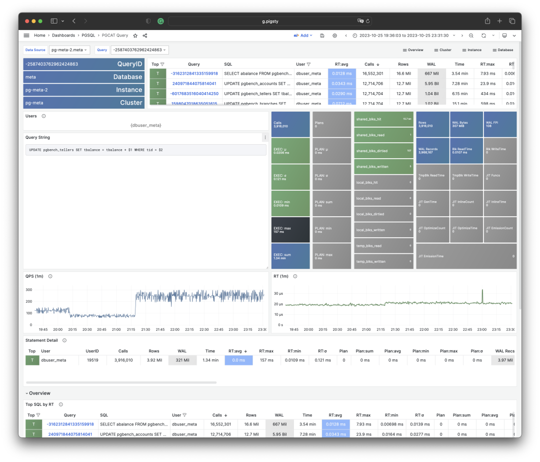
Visualizing a query group snapshot from the PGSS view

Compare at least two snapshots to measure activity over an interval. Match the same query-group key and account for counter resets or evicted entries before calculating differences.

A single snapshot describes accumulated work since that entry began collecting statistics. Interval differences are more useful for investigating a particular incident.

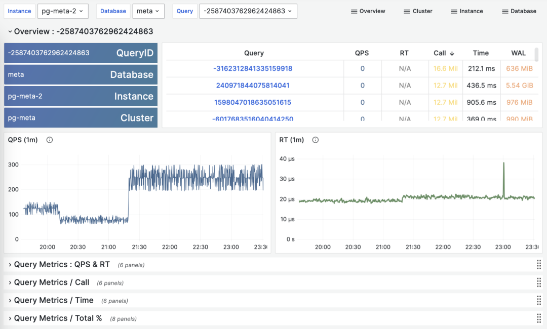
Calculating historical time-series metrics from multiple PGSS query group snapshots

The Pigsty deployment illustrated here took snapshots every 10 seconds of the top 256 queries by total time. With repeated samples of a cumulative metric M, we can calculate three derived metrics:

dM/dt: Derivative of metric M with respect to time, i.e., increment per second.

dM/dc: Derivative of metric M with respect to call count, i.e., average increment per call.

%M: Percentage of metric M in the overall workload.

These three types of metrics correspond exactly to the three types of macro optimization goals. The time derivative dM/dt reveals resource usage per second, typically used for resource consumption reduction optimization goals. The call count derivative dM/dc reveals resource usage per call, typically used for user experience improvement optimization goals. The percentage metric %M shows the percentage a query group occupies in the overall workload, typically used for workload balancing optimization goals.

Time Derivatives

Let’s first look at the first type of metrics: time derivatives. Here, the metrics M we can use include: calls, total_exec_time, rows, wal_bytes, shared_blks_hit + shared_blks_read, and blk_read_time + blk_write_time. Other metrics also have reference value, but let’s start with the most important ones.

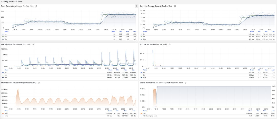
Visualizing time derivative metrics dM/dt

Calculating these metrics is actually quite simple, we just need to:

• First calculate the difference in metric value M between two snapshots: M2 - M1
• Then calculate the time difference between two snapshots: t2 - t1
• Finally calculate (M2 - M1) / (t2 - t1)

Production environments typically use data sampling intervals like 5s, 10s, 15s, 30s, 60s. For load analysis, we typically use 1m, 5m, 15m as common analysis window sizes.

For example, when we calculate QPS, we would calculate QPS for the last 1 minute, 5 minutes, and 15 minutes respectively. Longer windows provide smoother curves that better reflect long-term trends, but hide short-term fluctuation details and are not conducive to discovering momentary anomalies, so metrics of different granularities need to be viewed together.

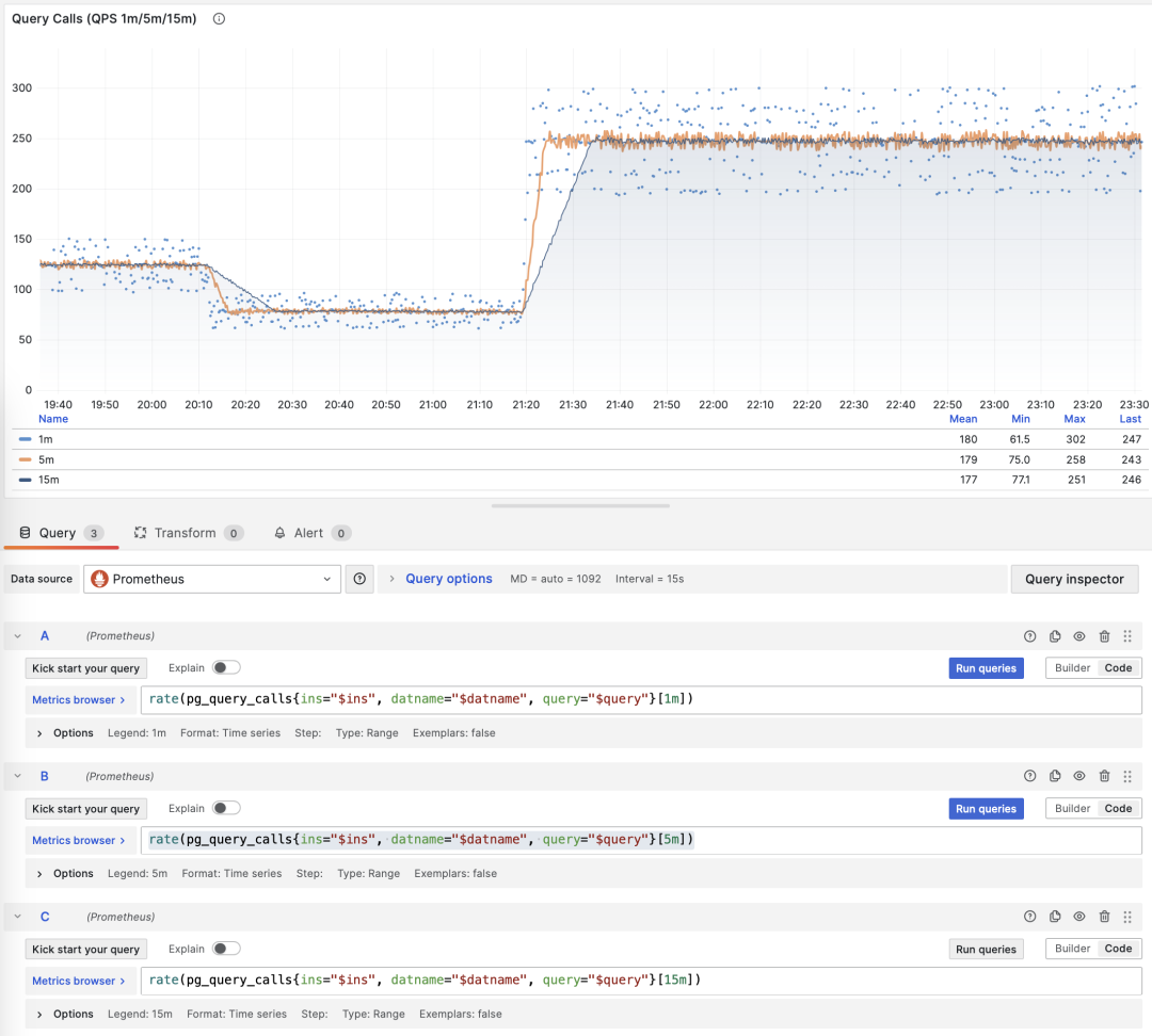
Showing QPS for a specific query group in 1/5/15 minute windows

For example, rate(pg_query_calls{}[1m]) calculates the one-minute QPS rate for each collected query-group series. To calculate a total, select the intended instance and sum its series.

QPS

When M is calls, the result of time differentiation is QPS, with units of queries per second (req/s). This is a very fundamental metric. Query QPS is a throughput metric that directly reflects the load situation imposed by business. If a query’s throughput is too high (e.g., 10000+) or too low (e.g., 1-), it may be worth attention.

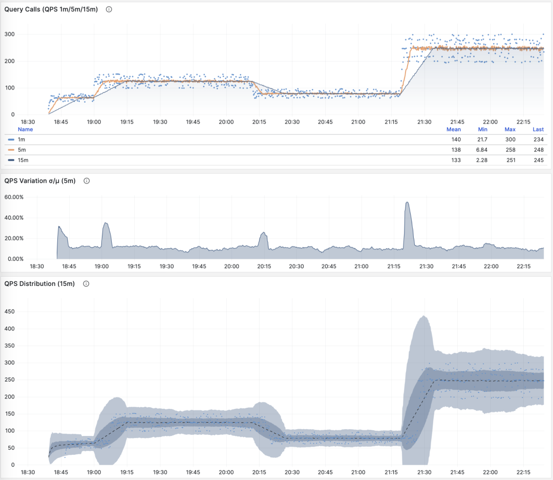
QPS: 1/5/15 minute µ/CV, ±1/3σ distribution

If we sum up all query groups’ QPS metrics (without exceeding PGSS collection range), we get the so-called “global QPS.” Another way to obtain global QPS is through client-side instrumentation, collection at connection pool middleware like PgBouncer, or using eBPF probes. But none are as convenient as PGSS.

Note that QPS metrics don’t have load-wise horizontal comparability. Different query groups may have the same QPS but vastly different per-query execution times. Even the same query group may produce dramatically different load levels at different times due to different execution plans. Execution time per second is a better metric for measuring load.

Execution Time Per Second

When M is total_exec_time (+ total_plan_time, optional), we get one of the most important metrics in macro optimization: execution time spent on query groups. Interestingly, this derivative has units of seconds/per second, so the numerator and denominator cancel out, making it actually a dimensionless metric.

For example, 2 s/s means that this query group accumulated two seconds of server execution time per second. Concurrent backends can produce this value even on one CPU core: elapsed execution time includes waits.

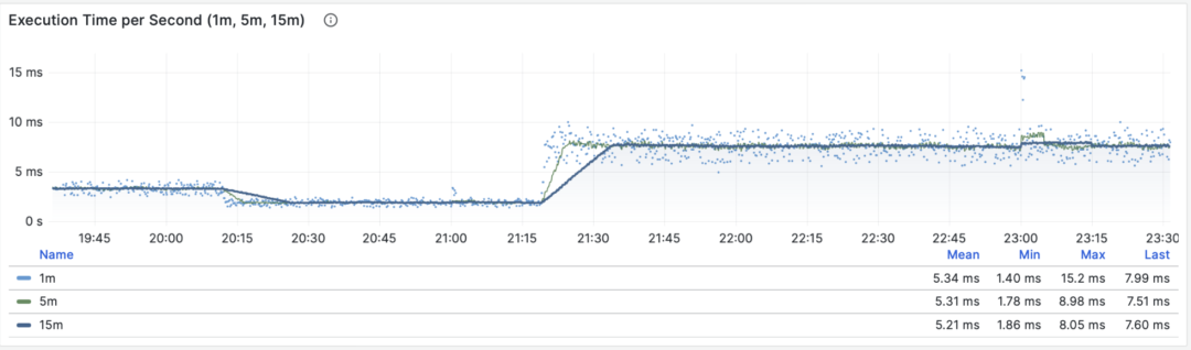
Execution time per second: 1/5/15 minute averages

Therefore, this value can also be understood as a percentage: it can exceed 100%, and in this perspective, it’s a metric similar to host load1, load5, load15, revealing the load level generated by this query group. If divided by CPU core count, you can even get a normalized query load contribution metric.

However, we need to note that execution time includes time waiting for locks and I/O. So it’s possible that query execution time is very long but has no impact on CPU load. For precise slow query analysis, we need to refer to wait events for further analysis.

Rows Per Second

When M is rows, the result is rows retrieved or affected per second. For a SELECT group, 10,000 rows/s describes the result-row rate. For an UPDATE or DELETE group, it describes affected rows, not data sent to clients.

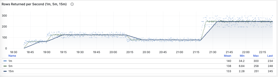
Rows retrieved or affected per second: 1/5/15 minute averages

Shared Buffer Access Bandwidth

When M is shared_blks_hit + shared_blks_read, we get the number of shared buffer blocks hit/read per second. If we multiply this by the default block size of 8KiB (rarely other sizes like 32KiB), we get the bandwidth of a query type “accessing” memory/disk: bytes per second.

For example, if a certain query type accesses 500,000 shared buffers per second, that’s 3.8 GiB/s of internal access data flow: this is significant load and might be a good optimization candidate. Perhaps you should examine this query to see if it deserves this “resource consumption.”

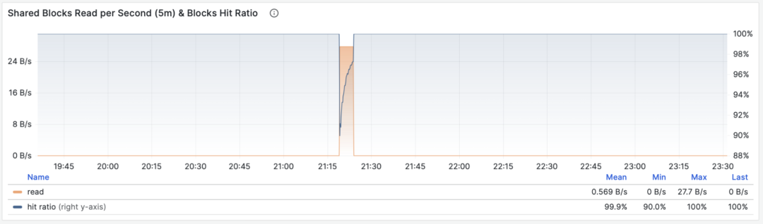
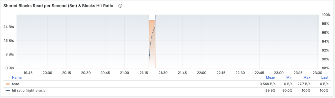
Shared buffer access bandwidth and buffer hit rate

Another valuable derived metric is buffer hit rate: hit / (hit + read). It can be used to analyze possible causes of performance changes — cache misses. Of course, repeatedly accessing the same blocks in the shared buffer pool doesn’t actually re-read, and even real reads might be from memory’s FS Cache rather than disk. So this is just a reference value, but it’s indeed a very important macro query optimization reference metric.

WAL Volume

When M is wal_bytes, we get the rate at which this query generates WAL, with units of bytes per second (B/s). This metric was introduced in PostgreSQL 13 and can quantitatively reveal the WAL size generated by queries: the more and faster WAL is written, the greater the pressure on disk flushing, physical/logical replication, and log archiving.

A typical example is: BEGIN; DELETE FROM xxx; ROLLBACK;. Such transactions delete lots of data, generate large amounts of WAL but perform no useful work. This metric can identify them.

WAL byte rate: 1/5/15 minute averages

The DELETE completes successfully before the explicit ROLLBACK undoes its transaction. PGSS records the successful statement, including the WAL it generated.

SELECT can also generate WAL when it sets hint bits. With data checksums or wal_log_hints enabled, the first such change to a page after a checkpoint can require a full-page image. See the WAL settings.

Check wal_fpi to determine whether full-page images explain WAL generated by a read-heavy workload.

Shared buffer dirty/writeback bandwidth

For versions below 13, shared buffer dirty/writeback bandwidth metrics can serve as an approximate lower substitute for analyzing query group write load characteristics.

I/O Time

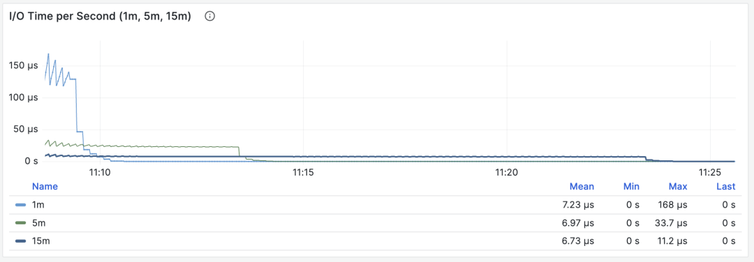
When M is blk_read_time + blk_write_time, convert milliseconds to seconds before taking the rate. The result is I/O time in seconds per second. Enable track_io_timing to collect these fields.

I/O time is very helpful for analyzing query spike causes

These timings include reads satisfied by the operating-system cache. Compare them with host disk metrics to distinguish cached reads from storage I/O.

Time derivative metrics dM/dt can show the overall workload inside a database instance/cluster, especially useful for resource usage optimization scenarios. But if your optimization goal is improving user experience, then another group of metrics — call count derivatives dM/dc — might be more meaningful.

Call Count Derivatives

For dM/dc, the denominator changes from elapsed time to the increase in call count. This gives average resource use per completed call.

This class of metrics is even more important than the former because it provides several core metrics directly related to user experience, such as the most important — query response time (RT, Response Time), or latency.

Calculating these metrics is also simple, we just need to:

• Calculate the difference in metric value M between two snapshots: M2 - M1
• Then calculate the difference in calls between two snapshots: c2 - c1
• Then calculate (M2 - M1) / (c2 - c1)

For PromQL implementation, call count derivative metrics dM/dc can be calculated using “time derivative metrics dM/dt”. For example, to calculate RT, you can use execution time per second / queries per second, dividing the two metrics:

rate(pg_query_exec_time{}[1m]) / rate(pg_query_calls{}[1m])

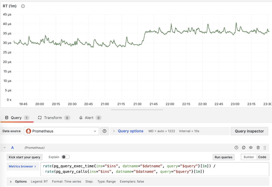
dM/dt can be used to calculate dM/dc

Call Count

When M is calls, differentiating with respect to itself is meaningless (result will always be 1).

Average Latency/Response Time/RT

Dividing the increase in total_exec_time by the increase in calls gives mean server execution time per call. Raw PGSS values produce milliseconds; the PromQL example above uses seconds. This is one part of client response time. Client-side measurements also include queueing, network, and application delays. Add planning time separately when planning statistics are enabled.

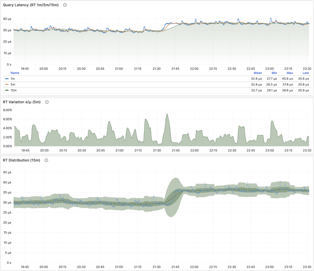
RT: 1/5/15 minute µ/CV, ±1/3σ distribution

The mean covers successful completed executions represented by the collected entries. pg_stat_statements.max limits how many groups PGSS retains. Check this coverage when comparing workloads.

Client instrumentation measures response time at the application boundary. PgBouncer and PostgreSQL 14+ also provide database-level timing aggregates. PGSS adds query-group detail.

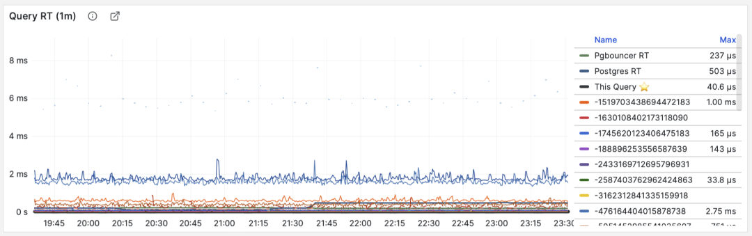
RT: Statement-level/Connection pool-level/Database-level

Compare RT for the same query group under similar conditions. If its usual mean is below 1 ms, a rise above 10 ms warrants investigation.

When failures occur, RT views are also helpful for pinpointing causes: if all queries’ overall RT slows down, it’s most likely related to resource insufficiency. If only specific query groups’ RT changes, it’s more likely caused by slow queries and should be investigated further. If RT changes coincide with application deployments, consider whether to rollback those deployments.

Additionally, in performance analysis, stress testing, and benchmarking, RT is also the most important metric. You can evaluate system performance by comparing typical queries’ latency performance in different environments (e.g., different PG major versions, different hardware, different configuration parameters) and continuously adjust and improve system performance based on this.

The mean and standard deviation of a sampled RT series show how interval averages vary. A percentile of those averages is not the P95 or P99 of individual query durations. Request-level percentiles require individual observations or a duration histogram.

RT is a useful measure of OLTP performance, alongside throughput and resource use.

Average Rows Per Call

When M is rows, the result is average rows retrieved or affected per call. For a point SELECT, this is usually a small result set; for a write statement, it is the number of affected rows.

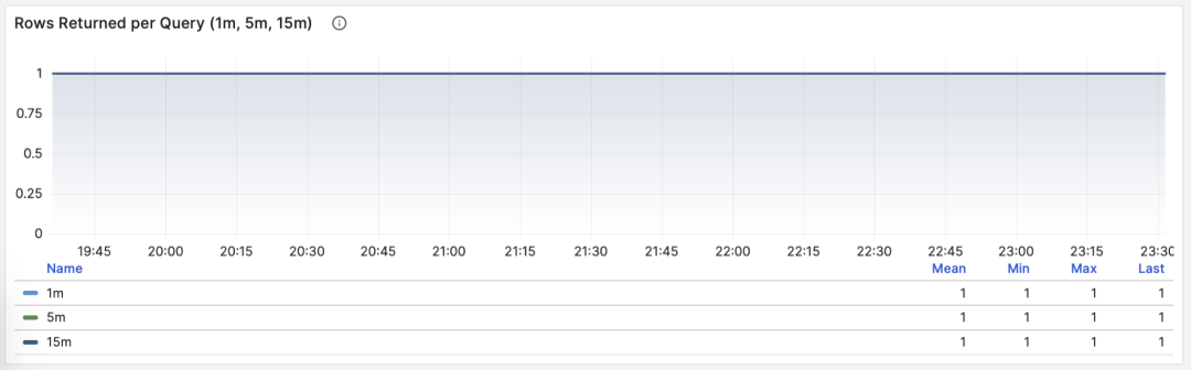
Point queries by primary key, average returned rows stable at 1

If a query group returns hundreds or even thousands of rows to clients per query, it should be examined. If this is intentional design, such as batch loading tasks/data dumps, then no action is needed. If these are requests initiated by applications/clients, there might be errors, such as statements lacking LIMIT restrictions or queries lacking pagination design. Such queries should be adjusted and fixed.

Average Shared Buffer Read/Hit

For shared_blks_hit + shared_blks_read, dM/dc gives shared-buffer accesses per query. Multiply by the block size, normally 8 KiB, to obtain bytes accessed per query (B/query). Repeated accesses count each time.

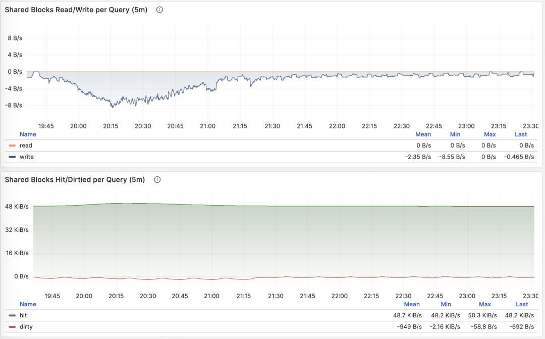
Average shared-buffer bytes accessed per query

Query average accessed data volume usually matches average returned rows. If your query only returns a few rows on average but accesses gigabytes of data blocks, you need special attention: such queries are very sensitive to data hot/cold states. If all blocks are in the buffer, performance might be acceptable, but if starting from disk cold, execution time might change dramatically.

A PostgreSQL buffer miss can still be satisfied by the operating-system cache. Compare host metrics, the pg_stat_kcache extension, or PostgreSQL 16’s pg_stat_io view to understand the underlying I/O.

Another pattern worth attention is sudden changes in this metric, which usually means this query group’s execution plan might have flipped/degraded, very worthy of attention and further study.

Average WAL Volume

When M is wal_bytes, we get the average WAL size generated per query. This is a field newly introduced in PostgreSQL 13. This metric can measure query change footprint size and calculate read/write ratios and other important evaluation parameters.

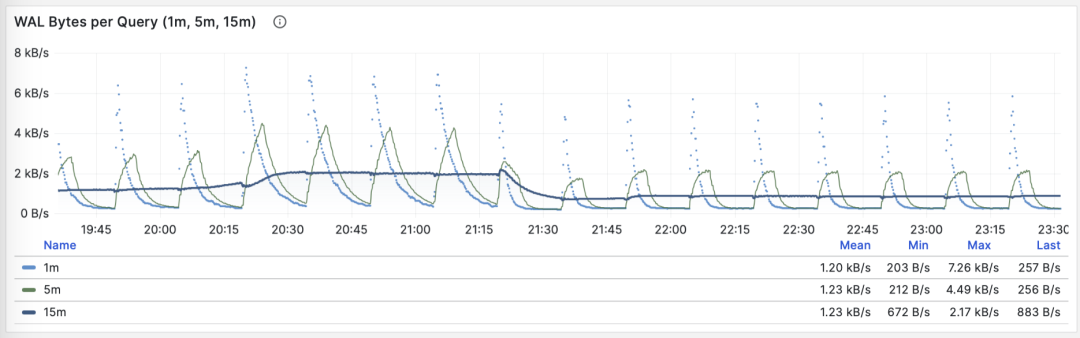
Stable QPS but periodic WAL fluctuations, inferred to be FPI influence

Another use is checkpoint optimization: if you observe periodic fluctuations in this metric (period approximately equal to checkpoint_timeout), you can optimize the amount of WAL generated by queries by adjusting checkpoint intervals.

dM/dc describes the average cost of one call. Use it to assess a query change, then check the workload totals to measure the overall effect.

dM/dc metrics like these provide important absolute value metrics, but to find which queries have the greatest potential optimization benefits, you need %M percentage metrics.

Percentage Metrics

Now let’s study the third type of metrics: percentage metrics. That is, the proportion a certain query group occupies relative to the overall workload.

Percentage metrics M% provide us with the proportion of a certain query group relative to the overall workload, helping us identify “major players” in frequency, time, I/O time/count, find query groups with the greatest potential optimization benefits, and serve as important basis for priority assessment.

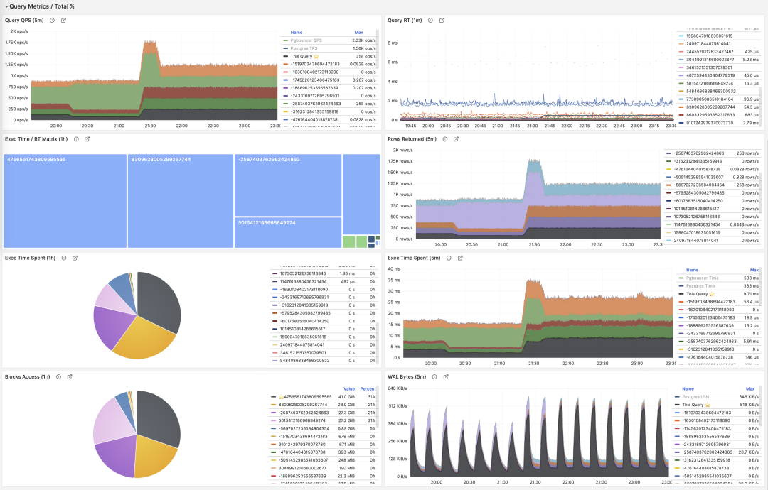
Common percentage metrics %M overview

A query group at 1,000 QPS might account for only 3% of calls, or more than 50%. If many of those calls are redundant, removing them can reduce database work. For expensive queries, compare their share of execution time or I/O as well as their share of calls.

A common optimization strategy is: first sort all query groups by the important metrics mentioned above: calls, total_exec_time, rows, wal_bytes, shared_blks_hit + shared_blks_read, and blk_read_time + blk_write_time dM/dt values over a period of time, take TopN (say N=10 or more), and add them to the optimization candidate list.

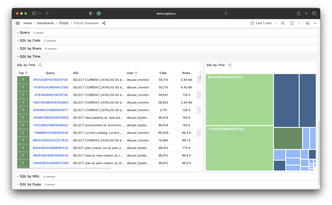
Selecting TopSQL for optimization by specific criteria

Then, for each query group in the optimization candidate list, analyze their dM/dc metrics in turn, combined with specific query statements and slow query logs/wait events for analysis, decide whether this is a query worth optimizing. For queries decided (Plan) to optimize, you can use techniques introduced in the subsequent “micro optimization” article for tuning (Do), and use monitoring systems to evaluate optimization effects (Check), summarize and analyze before entering the next PDCA Deming cycle, continuing management optimization.

Besides taking TopN on metrics, visualization can also be used. Visualization greatly helps identify “major contributors” from workloads. Complex judgment algorithms might not match human DBAs’ intuition for monitoring pattern recognition. To form a sense of proportion, we can use pie charts, tree maps, or stacked time series charts.

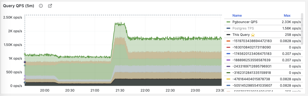
Stacking QPS of all query groups

For example, we can use pie charts to identify queries with the highest time consumption/IO usage in the past hour, use 2D tree maps (size represents total time consumption, color represents average RT) to show an additional dimension, and use stacked time series charts to show how proportions change over time.

We can also directly analyze current PGSS snapshots, sort by different concerns, and select queries to be optimized according to your own criteria.

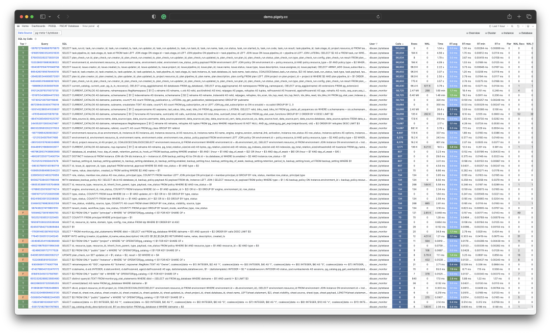
I/O time is very helpful for analyzing query spike causes

Summary

Finally, let’s summarize the content above.

PGSS provides rich metrics, among which the most important cumulative metrics can be processed in three ways:

dM/dt: Derivative of metric M with respect to time, revealing resource usage per second, typically used for resource consumption reduction optimization goals.

dM/dc: Derivative of metric M with respect to call count, revealing resource usage per call, typically used for user experience improvement optimization goals.

%M: Percentage metrics show the percentage a query group occupies in the overall workload, typically used for workload balancing optimization goals.

Usually, we select high-value candidate optimization queries based on %M: percentage metric Top queries, and use dM/dt and dM/dc metrics for further evaluation, confirming whether there’s optimization space and feasibility, and evaluating post-optimization effects. This cycles continuously.

After understanding macro optimization methodology, we can use this approach to locate and optimize slow queries. Here’s a specific example of Using Monitoring Systems to Diagnose PG Slow Queries. In the next article, we’ll introduce experience and techniques for PostgreSQL query micro optimization.

References

[1] PostgreSQL HowTO: pg_stat_statements by Nikolay Samokhvalov

[2] pg_stat_statements

[3] Using Monitoring Systems to Diagnose PG Slow Queries

[4] How to Monitor Existing PostgreSQL (RDS/PolarDB/Self-built) with Pigsty?

[5] Pigsty v2.5 Released: Ubuntu/Debian Support and Monitoring Redesign/New Extensions

[6] PostgreSQL Monitoring System Pigsty Overview

4 - Monitor Existing PostgreSQL with Pigsty: RDS, PolarDB, and Self-Hosted Databases

This tutorial describes Pigsty and Alibaba Cloud services as used in September 2023. Commands, prices, and dashboard details reflect that period.

Pigsty is a PostgreSQL distribution. You can also use it solely to monitor PostgreSQL and hosts. This tutorial uses Alibaba Cloud as an example: install Pigsty on one ECS instance, then connect existing PolarDB and RDS for PostgreSQL databases.

Video tutorial

Procedure

The tutorial has four steps:

1. Create an ECS instance for Pigsty.
2. Install the full single-node Pigsty environment on it.
3. Configure the monitoring user, schemas, views, and access lists in PolarDB or RDS.
4. Register the database instances with Pigsty monitoring.

At the time of writing, the example required an Alibaba Cloud account with a balance above CNY 100 for pay-as-you-go resources. The example resources cost about CNY 4 per hour.

Why add this monitoring system?

Cloud providers already offer RDS monitoring. I needed more metrics to analyze slow queries, diagnose faults, and assess capacity, so I added this system.

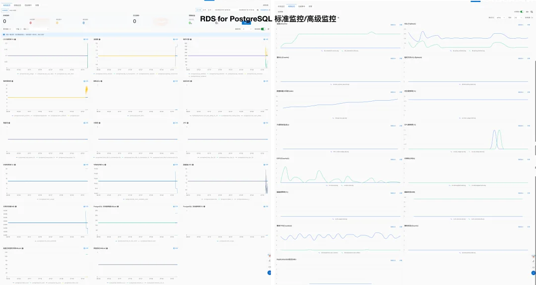
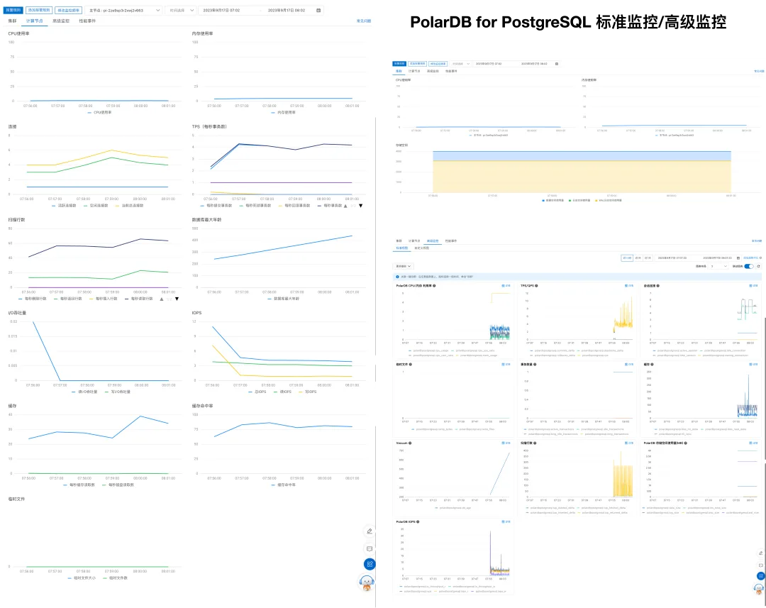
Pigsty uses Grafana and Prometheus, packaged as an INFRA module that can be installed together. Components managed by Pigsty are added to monitoring: hosts, HAProxy, PostgreSQL, PgBouncer, etcd, Redis, MinIO, and the monitoring infrastructure itself. The supplied dashboards and alert rules show system status and support troubleshooting.

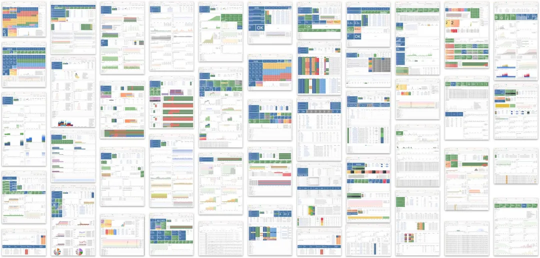
At the time of this article, a full deployment used more than 3,000 kinds of metrics for databases and supporting components. Dashboards organize the data by cluster, instance, and object. They show activity on tables, indexes, and functions, as well as cluster totals. Links switch between views; the time selector compares current activity with historical trends.

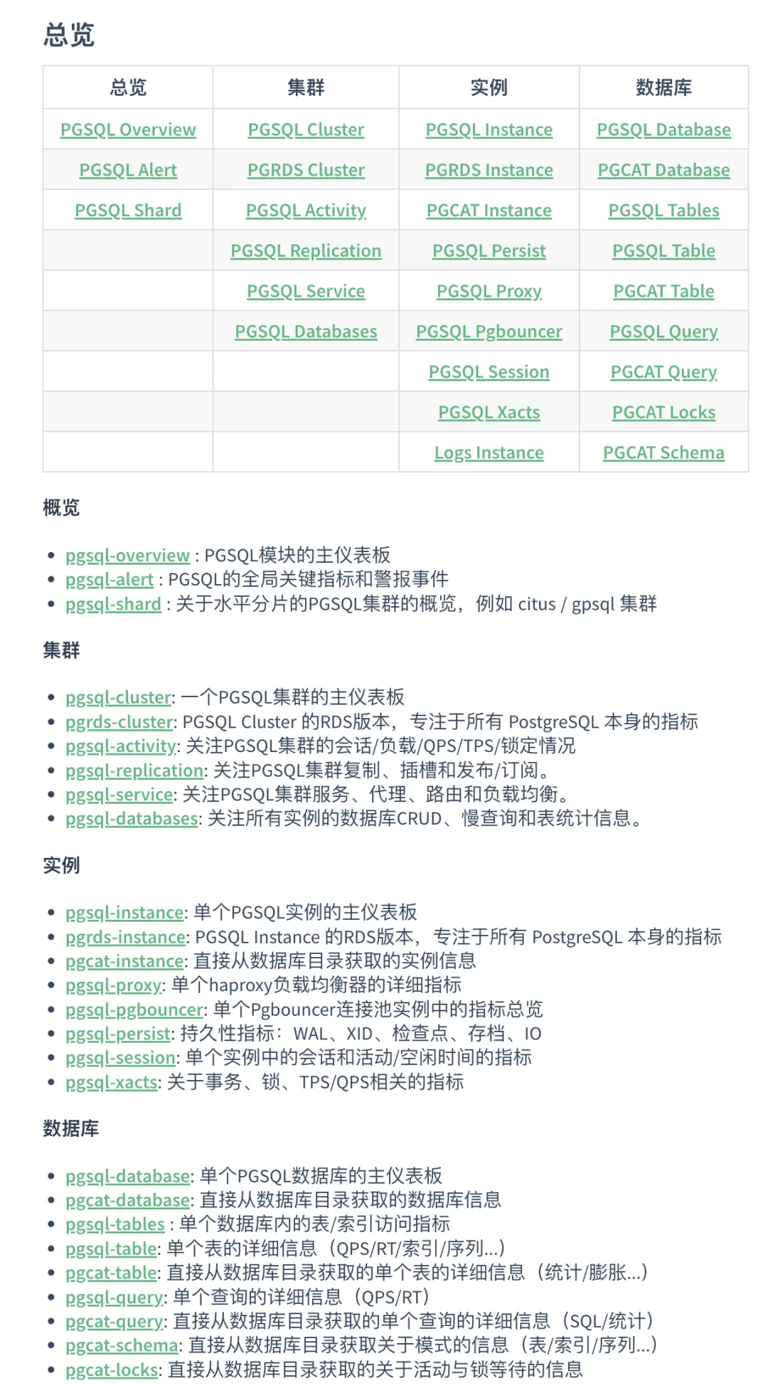
For an existing PostgreSQL database, especially a managed cloud service, available data depends on the service’s access interfaces. This setup usually lacks host, high-availability, connection-pool, and native database log data. It mainly uses PostgreSQL’s own metrics.

Explore the public demo to see the monitoring interface.

Create an ECS instance

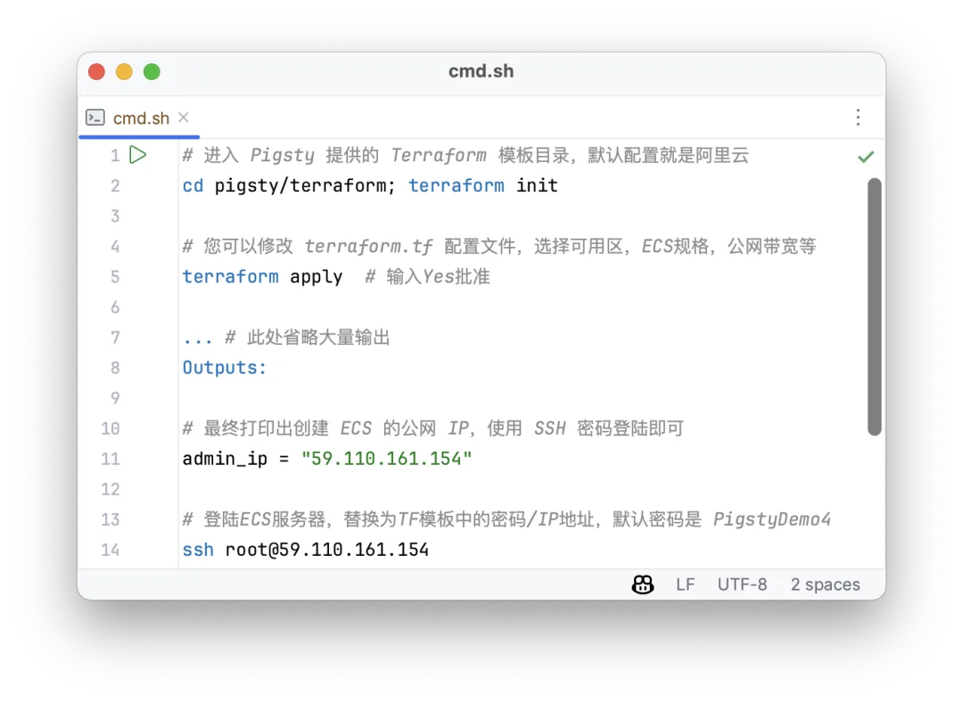
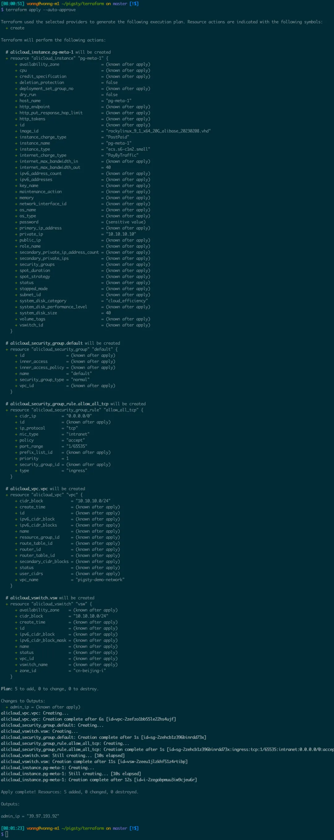
The setup shown here used an x86_64 ECS instance running EL 7–9, with Rocky Linux 8.6 or 9.1 recommended at the time. The minimum size was one CPU and 2 GB of memory. You could create it in the cloud console or use Pigsty’s Terraform template.

The demonstration template assigned the private address 10.10.10.10, the example password PigstyDemo4, and a public IP address for access.

Install single-node Pigsty on ECS

After logging in to ECS, the installation workflow was:

bash -c "$(curl -fsSL https://get.pigsty.cc/latest)"  # Download Pigsty
cd ~/pigsty
./bootstrap                                        # Download the offline packages
./configure                                        # Configure Pigsty
vi pigsty.yml                                      # Set passwords and other local settings
./install.yml                                      # Install the single-node environment

With the offline packages, the full installation took about ten minutes. The current procedure is in the Pigsty installation guide.

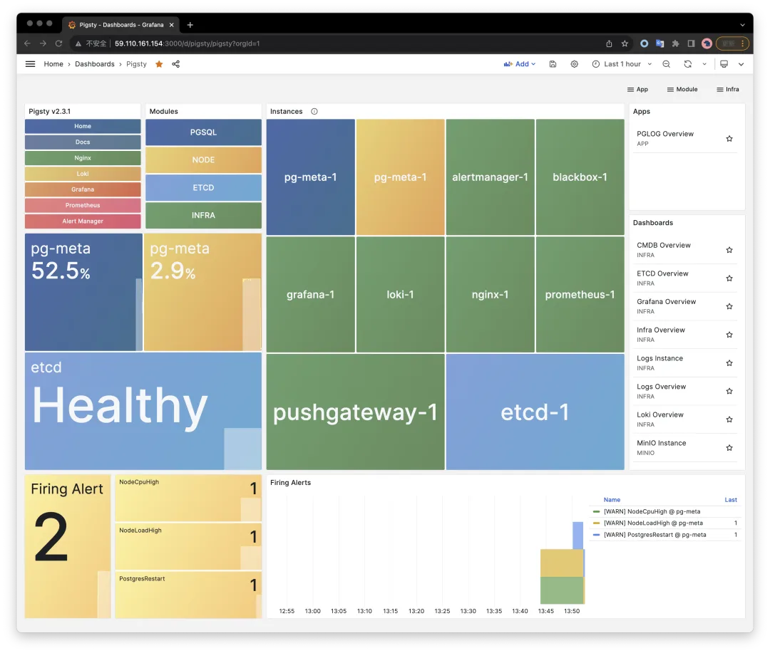
After installation, Grafana was available on port 3000 of the ECS public address. It included monitoring for the new environment itself. The example installation used the default Grafana credentials admin / pigsty.

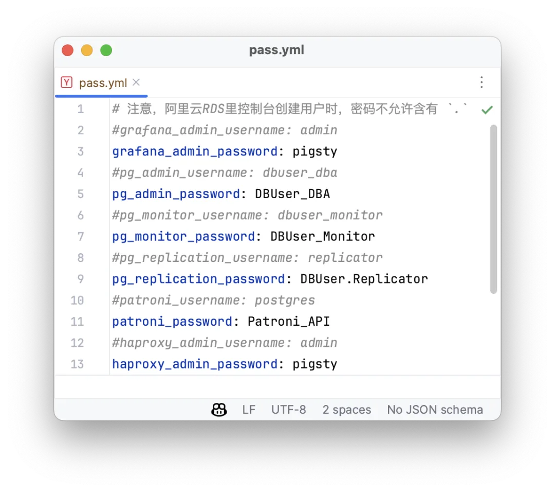
Use a domain name and HTTPS for the web interface. Replace the example passwords and restrict access to the monitoring system.

Configure PolarDB or RDS for monitoring

The exporter needs a connection URL that it can reach from ECS, a monitoring account with the required read permissions, and any extensions used by the selected collectors.

For the PolarDB example:

1. Create the cluster in a network reachable from ECS. This example used the same availability zone and subnet.
2. Create the privileged administration account dbuser_dba for initial configuration.
3. Add the ECS private address, 10.10.10.10, to the cluster access allowlist.
4. Create a database, named test in this example.

Connect as the administrator to configure the monitoring role. Substitute your cluster endpoint and use a password prompt:

psql -h your-cluster.polardbpg.rds.aliyuncs.com -p 1921 -U dbuser_dba -d test -W

Create a dedicated monitoring user with this account, or create it through the cloud console.

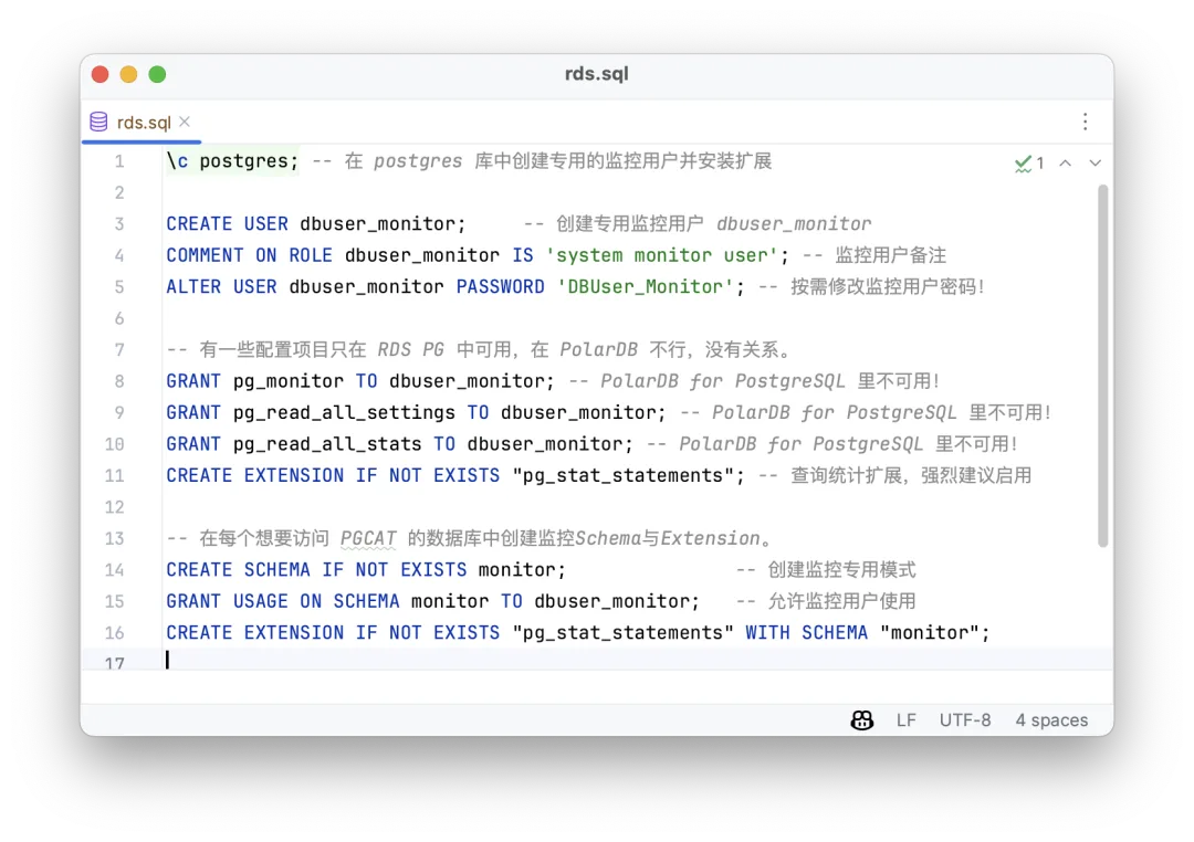
Install pg_stat_statements to collect query-level statistics, including call counts and execution time.

Register existing databases

To add RDS and PolarDB instances, provide their identities and connection settings in pigsty.yml. In the version used here, all.children.infra.vars.pg_exporters was a dictionary: each key was a unique local exporter port, and each value described a target database instance.

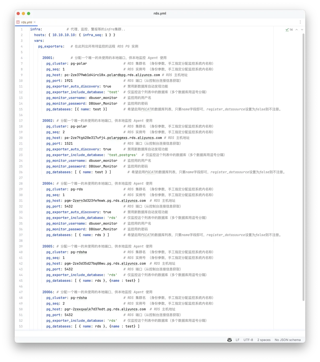
This example registered three clusters:

• pg-polar: a PolarDB cluster with one primary and one replica.
• pg-rds: a basic, single-node RDS for PostgreSQL instance.
• pg-rdsha: a high-availability RDS cluster with an additional read-only node.

The screenshot shows the configuration. Usually, the fields to change were pg_cluster, pg_seq, and pg_host, plus pg_port when the port was not 5432. Other settings could be overridden as needed.

After defining the targets, add each cluster to monitoring:

bin/pgmon-add pg-polar
bin/pgmon-add pg-rds
bin/pgmon-add pg-rdsha

The three clusters then appear in Pigsty:

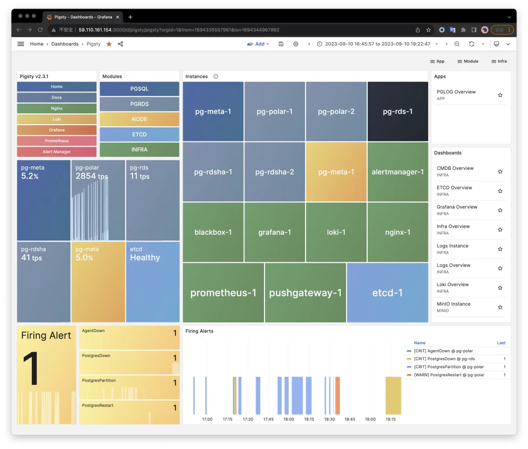
Click a cluster or instance name in light blue to open its PGRDS dashboard.

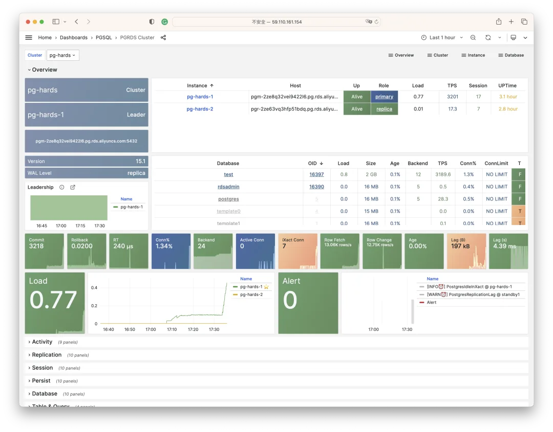
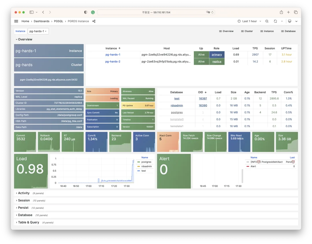
The opening screen shows cluster members, health, the database list and navigation, and 13 core metrics. Click a panel to inspect the details.

Links within charts let you move between PGRDS Cluster and PGRDS Instance, from a cluster overview to one instance and back.

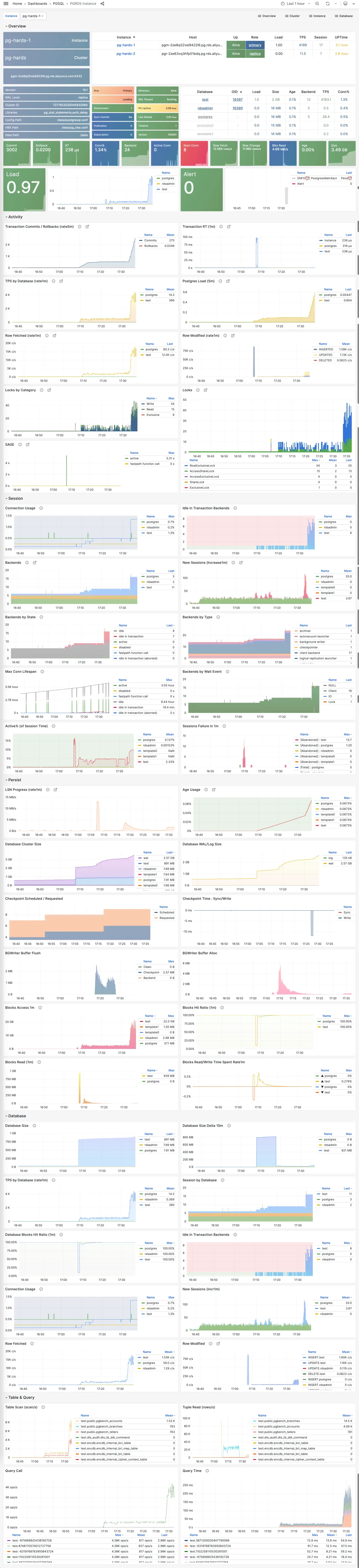
The Overview and Database dashboards remain available. They show details such as QPS and response time for each query class, or reads and writes on each table.

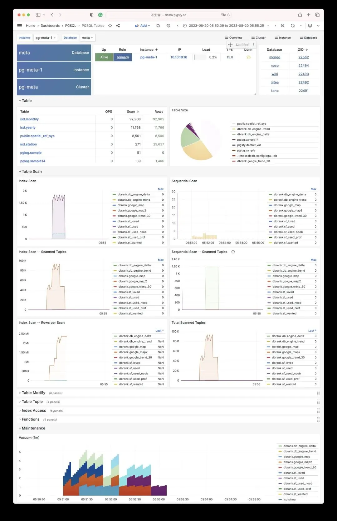
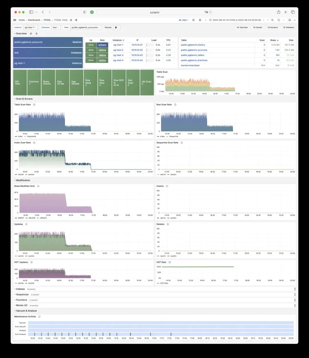
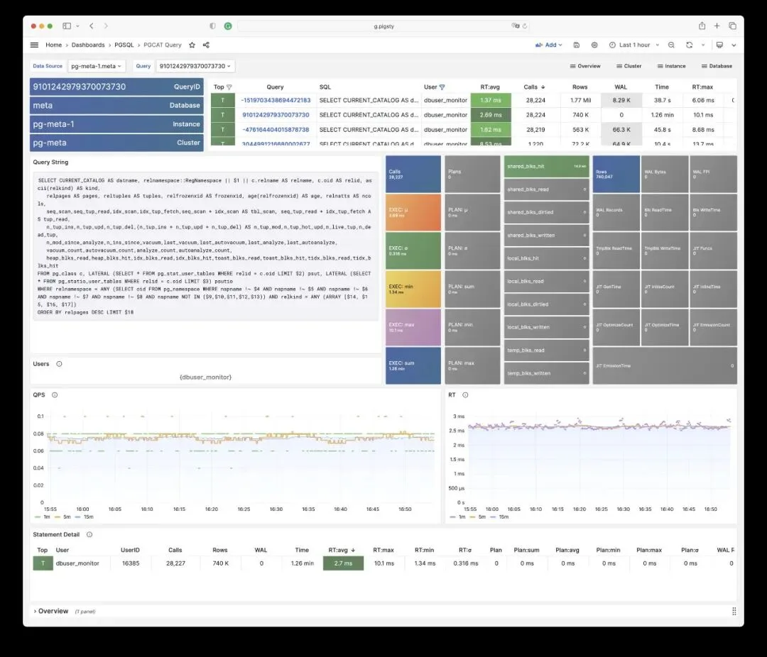
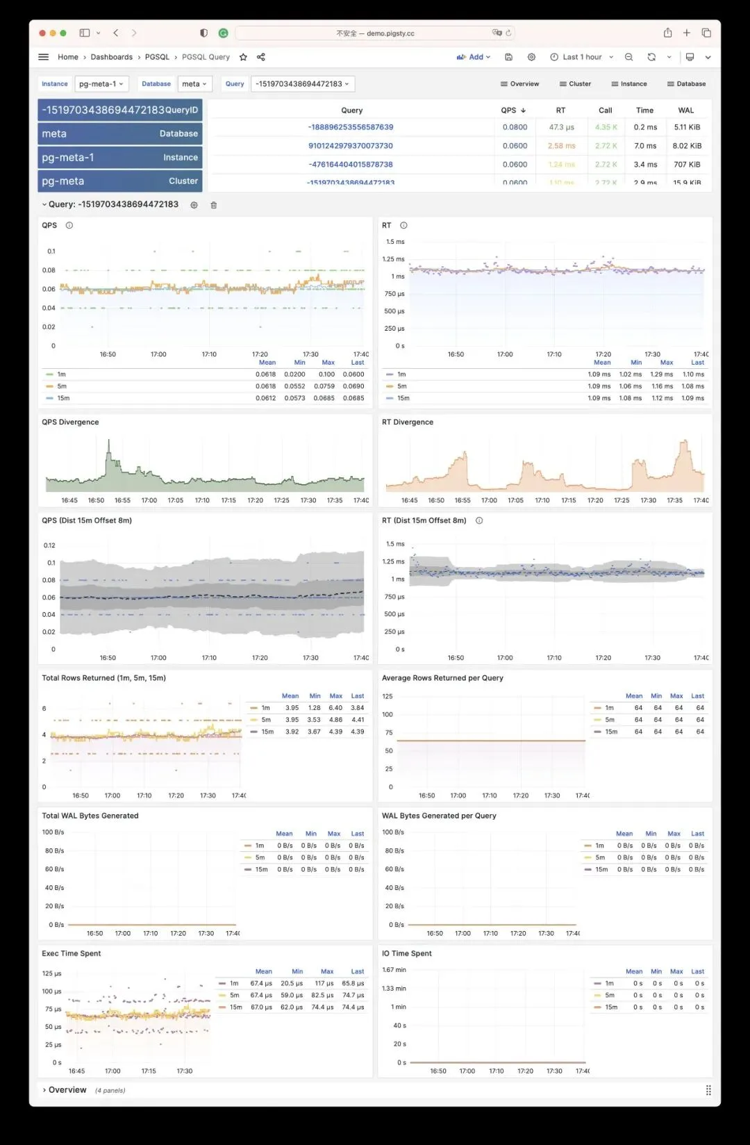
Pigsty can also query the database catalog directly through an optional data source. This provides views of current lock waits and top SQL statements.

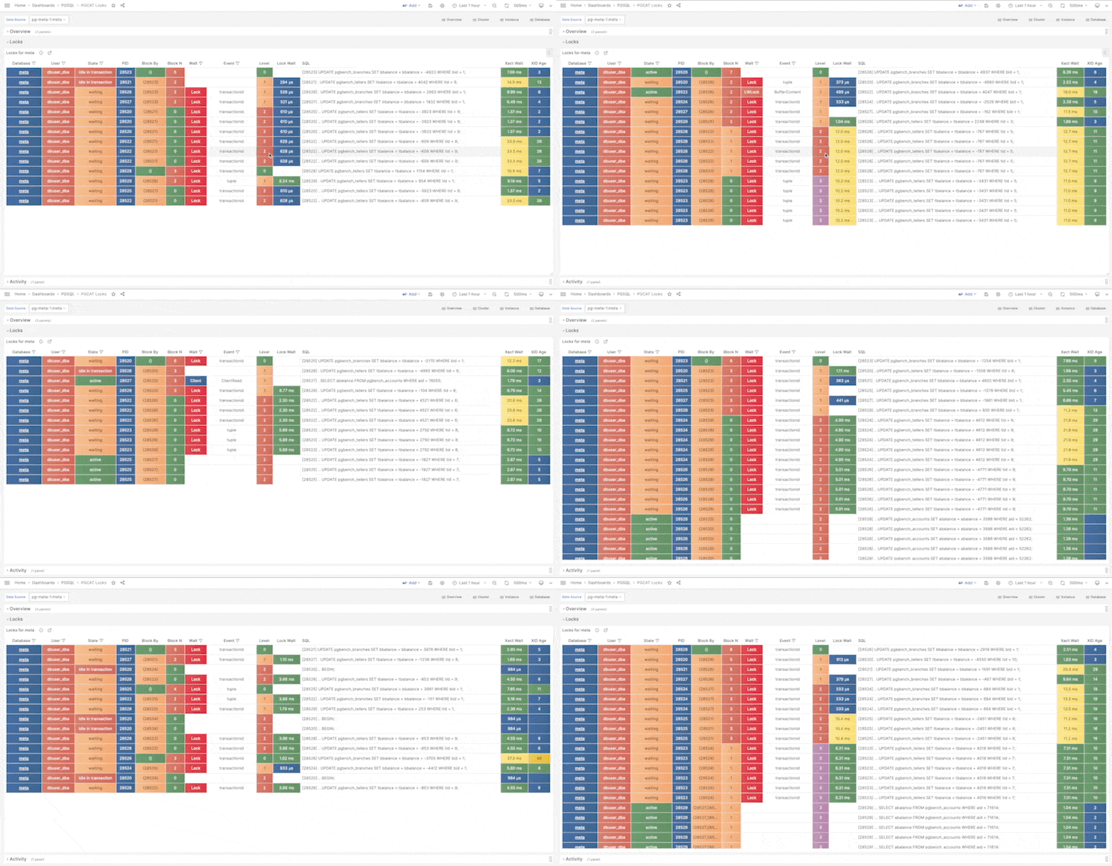
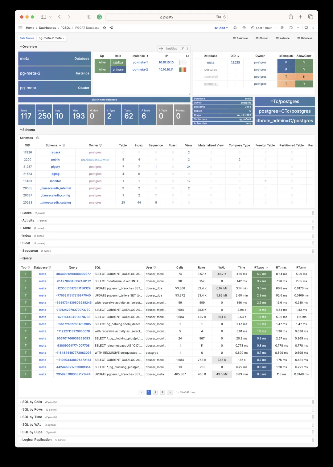
For more detail, see the Pigsty documentation, explore the demo, or watch the video tutorial.

To join the PGSQL × Pigsty discussion group, search for pigsty-cc on WeChat and contact the Pigsty assistant.

5 - Diagnose PostgreSQL slow queries

This walkthrough uses the Pigsty sandbox and dashboards from February 2021.

Slow queries occupy connections, hold locks, and consume CPU and I/O. On a standby, a long query can conflict with WAL replay. PostgreSQL can delay replay or cancel the conflicting query, depending on its standby settings. See hot standby conflicts.

Monitoring helps you find the affected query and compare its behavior before and after a change.

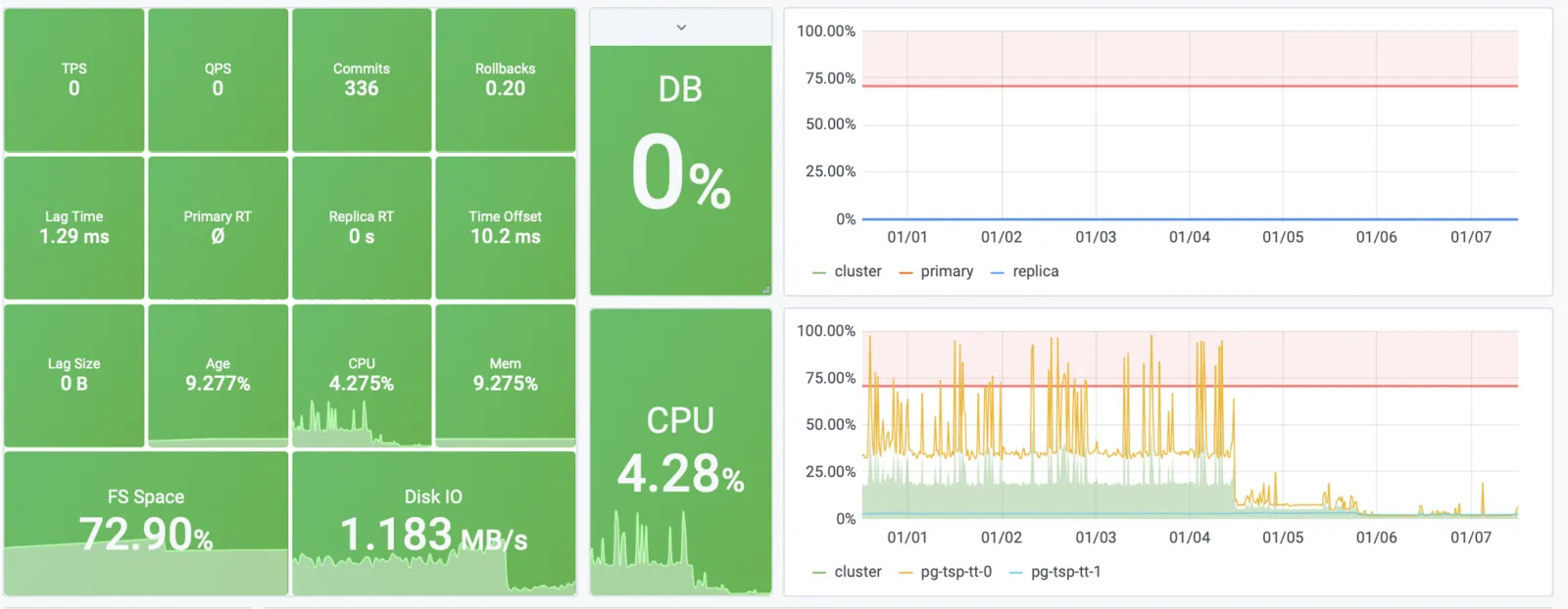
In this example, query optimization reduced CPU use from about 40% to 4%.

Collect query statistics and logs

The pg_stat_statements extension groups similar statements. It records call counts, execution times, rows retrieved or affected, and I/O statistics. To enable it:

1. Add pg_stat_statements to shared_preload_libraries.
2. Restart PostgreSQL.
3. Run CREATE EXTENSION pg_stat_statements in the database where you will read the statistics.

A query ID identifies a normalized statement. It does not identify one execution or guarantee one execution plan. Column names vary by PostgreSQL version; use the matching pg_stat_statements reference.

Use log_min_duration_statement to log statements whose duration reaches a threshold. These logs help explain individual slow executions. Choose the threshold for the workload: logging every statement increases log volume and collection overhead.

A cumulative average can hide a recent regression. Take repeated samples to compare response time, call rate, and I/O over the incident interval. A slow-query threshold should reflect the application’s latency requirement. A frequent point lookup and an occasional batch query need different thresholds.

Reproduce the problem in a sandbox

This experiment deliberately removes an index. Run it in a disposable pgbench database.

The historical Pigsty sandbox used make ri, make ro, and make rw to initialize and exercise the pg-test cluster. The following commands apply write and read loads through its service ports:

# Write load: 50 transactions per second
while true; do pgbench -nv -P1 -c20 --rate=50 -T10 postgres://test:test@pg-test:5433/test; done

# Read load: 1000 transactions per second
while true; do pgbench -nv -P1 -c40 --select-only --rate=1000 -T10 postgres://test:test@pg-test:5434/test; done

Run each load in its own terminal. On the primary, remove the primary key:

ALTER TABLE pgbench_accounts DROP CONSTRAINT pgbench_accounts_pkey;

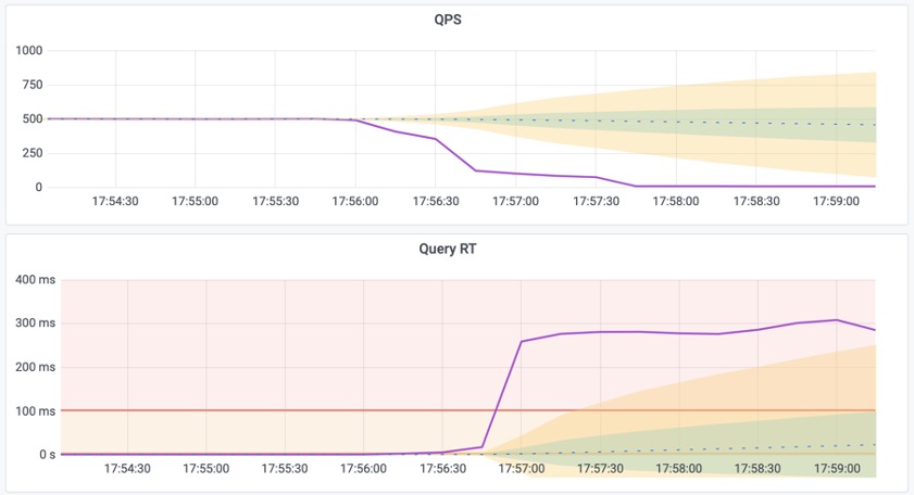
The point lookup loses its index. In this test, average response time increased from about 1 ms to 300 ms. One replica’s QPS fell from 500 to 7.

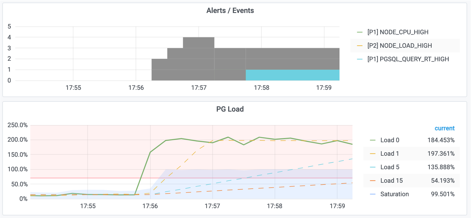
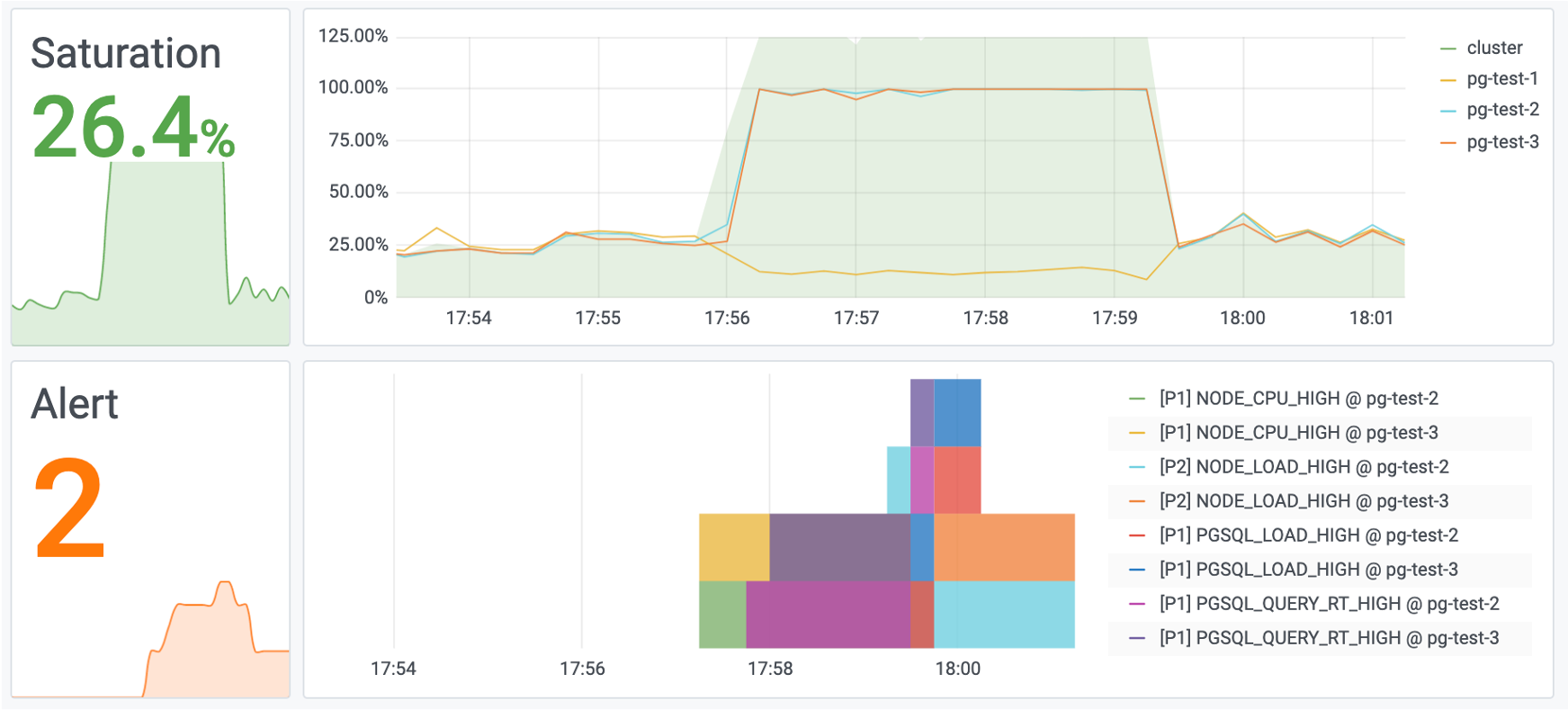
The cluster load also increased and triggered alerts.

Find the query

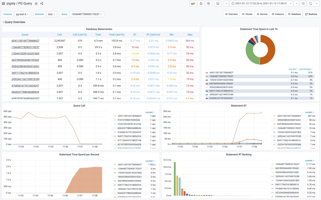
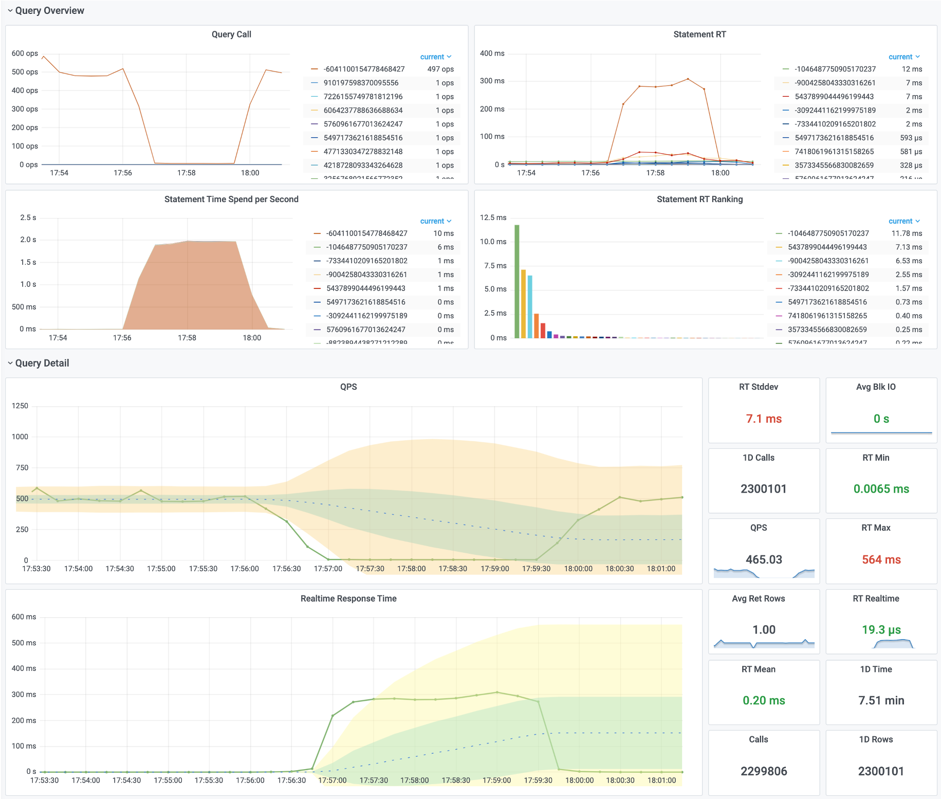
Open PG Cluster to identify the affected instance. In PG Query, look for statements whose response time and share of execution time increased.

In this example, query ID -6041100154778468427 changed from about 17 μs to 280 ms, while its QPS fell from 500 to 7.

Open PG Query Detail for this query ID to find the SQL:

SELECT abalance FROM pgbench_accounts WHERE aid = $1;

Test the cause

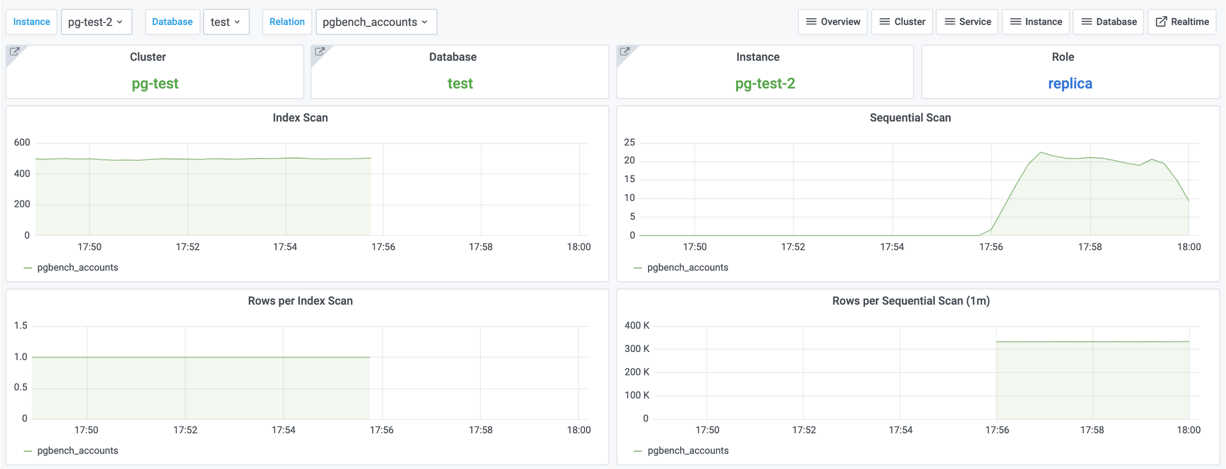
The statement retrieves one account by aid. In PG Table Catalog, check whether that column has an index. In PG Table Detail, compare index scans and sequential scans on pgbench_accounts.

In this experiment, index scans fell to zero and sequential scans increased after the primary key was removed. This supports the missing-index diagnosis.

Apply and verify the fix

Restore an index on aid in the sandbox:

CREATE UNIQUE INDEX ON pgbench_accounts (aid);

This restores the lookup path. It does not recreate the primary-key constraint removed earlier.

Compare the same workload and time intervals before and after the change. Record query latency, throughput, and resource use. Stop the test load when the experiment is complete.

6 - The First Pigsty Release

This article describes Pigsty at its January 2021 release.

Today, I released Pigsty.

Official website: pigsty.cc

What is Pigsty?

Pigsty monitors large PostgreSQL fleets and automates the deployment of highly available clusters. It is free, open-source software built on open-source components.

I wanted to reduce the manual work of managing PostgreSQL through a shared monitoring interface and deployment process.

Monitoring

I needed to manage a large PostgreSQL fleet. After trying several open-source and commercial monitoring products, I could not find one that met my needs, so I began building Pigsty.

The interface uses Grafana. At its first release, it contained more than 30 dashboards, over a thousand panels, and about 180,000 lines of JSON configuration, covering databases and infrastructure.

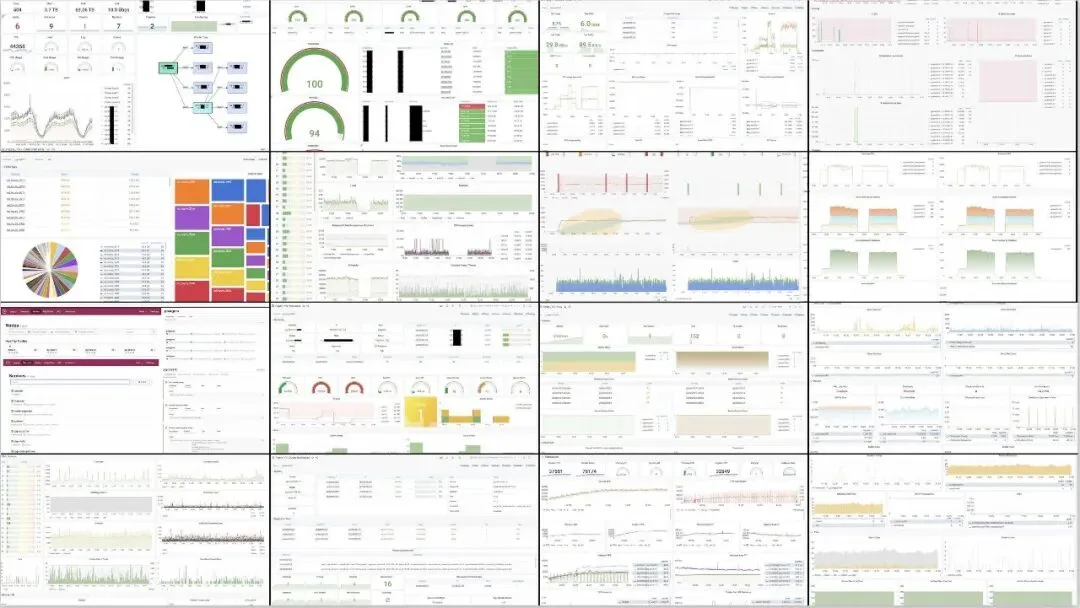
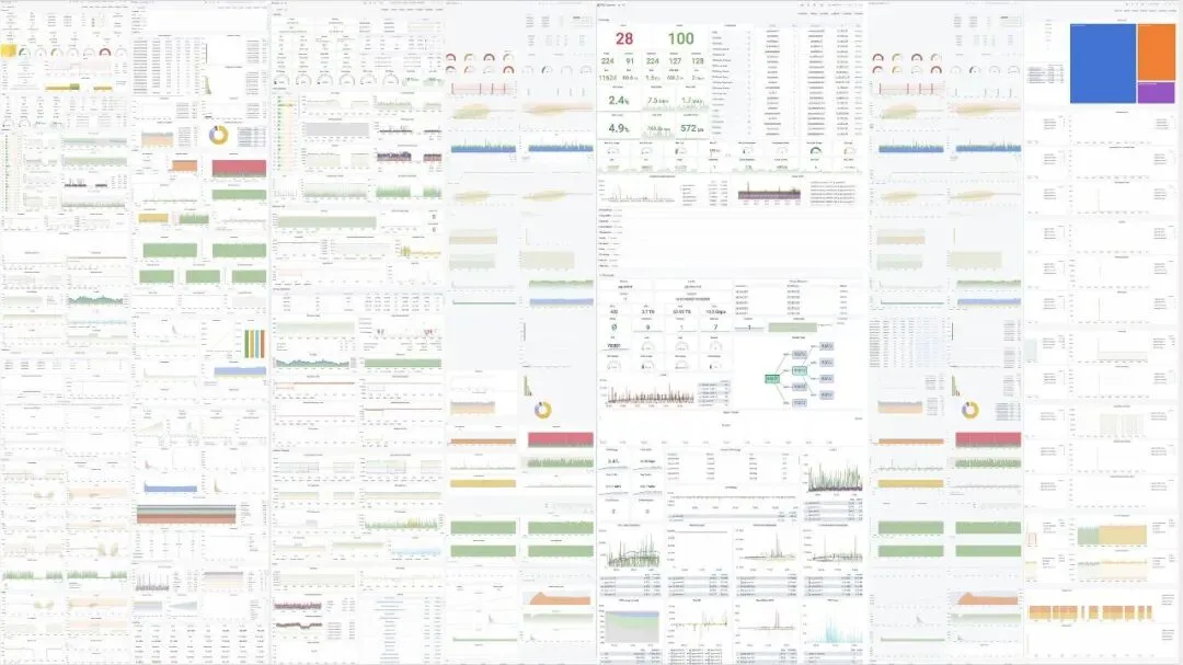
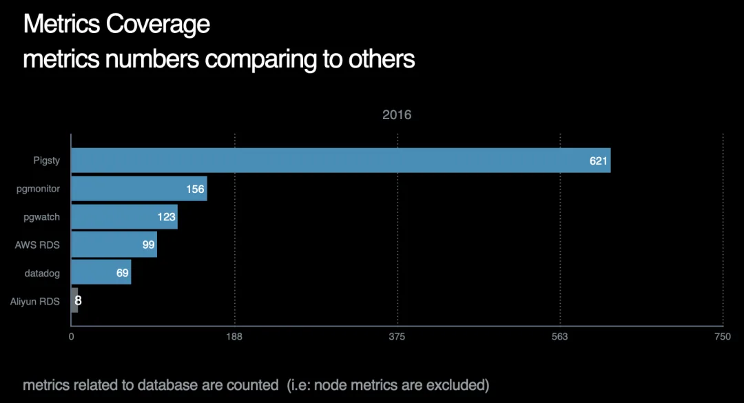
This version provided nearly 1,200 monitoring metrics. They show fleet-wide totals and let users inspect reads and writes on individual database objects.

Cluster provisioning

Distributing and demonstrating a monitoring system requires a database environment. Existing installations vary, so I included database provisioning in Pigsty.

The deployment combines replication, failover, traffic proxies, connection pooling, service discovery, and basic privilege configuration. This reduces the work of configuring each component separately.

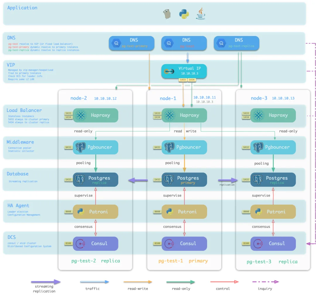
Fill in the configuration file, and Pigsty creates the database cluster it describes.

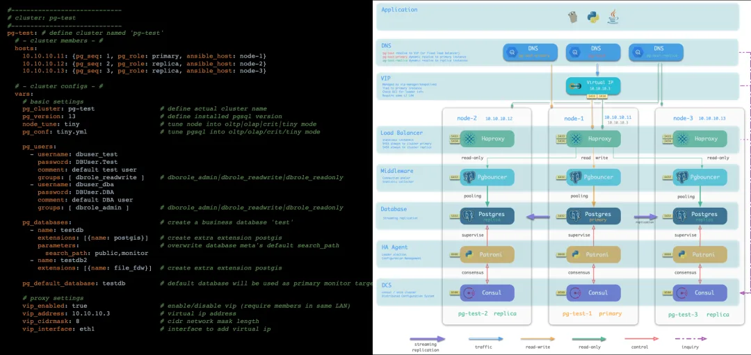
More than 130 settings describe the database and infrastructure. Declarative configuration and idempotent execution manage physical and virtual machines as infrastructure code, with a workflow similar to Kubernetes.

Open-source components and license

This release used the Apache 2.0 license, with a professional edition and optional commercial support also available. Issues, pull requests, donations, and sponsorship were welcome.

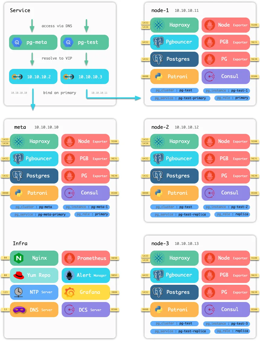
Monitoring uses Prometheus, Grafana, Alertmanager, and exporters. It also includes Nginx, Dnsmasq/CoreDNS, NTP/Chrony, Consul/etcd, and other infrastructure components. These can integrate with an existing monitoring environment.

Provisioning uses Ansible to deploy PostgreSQL, PgBouncer, Patroni, HAProxy, and Keepalived. Deployment logic is packaged as Ansible roles for integration and customization.

Try Pigsty

Pigsty provides English and Chinese documentation, a public demo, and a local Vagrant sandbox. At its first release, these commands created a sandbox with database clusters and monitoring infrastructure on a laptop:

make up          # Start the Vagrant virtual machines
make ssh         # Configure SSH access to the virtual machines
make init        # Initialize Pigsty
sudo make dns    # Add static Pigsty DNS entries; optional, requires sudo
make mon-view    # Open Pigsty; sandbox default credentials: admin / admin

Production environments use the same deployment process, with configuration adapted to their hosts, networks, and database requirements.

Project links

• Chinese documentation
• English documentation
• Public demo
• GitHub repository

7 - Golden Monitoring Metrics: Errors, Latency, Throughput, Saturation

Written in 2020. The metric counts and examples describe the deployment at that time.

Preface

Operating a database is like driving a car: both require attention to a dashboard.

Metrics show the current state and help you decide when to act.

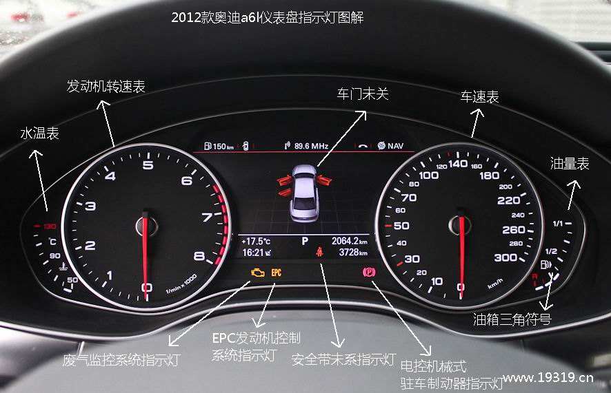
Cars have many metrics: speed, tire pressure, torque, brake pad wear, various temperatures, and so on - all kinds of different ones.

But human attention span is limited, and the dashboard is only so big.

So, metrics can be divided into two categories:

• Ones you will look at: Golden metrics / Key metrics / Core metrics
• Ones you won’t look at: Black box metrics / Cold metrics

Golden metrics are those few critical core data points that need constant attention (or have an autopilot system/alarm system maintain constant attention for you), while cold metrics are usually only looked at during troubleshooting. Troubleshooting and post-mortems require restoring the scene as much as possible, so the more black box metrics the better. It’s very frustrating when you need them but don’t have them.

Today let’s talk about PostgreSQL’s core metrics. What are the core metrics for databases?

Database Metrics

Before discussing database core metrics, let’s take a look at what metrics are available.

avg(count by (ins) ({__name__=~"pg.*"}))
avg(count by (ins) ({__name__=~"node.*"}))

In the deployment used for this article, these queries found more than 1,000 PostgreSQL series and 2,000 host series per instance.

These series support investigation and visualization.

But for daily management, only a few core metrics are needed.

With thousands of available metrics, which ones are the core metrics?

Core Metrics

Based on experience and usage frequency, continuously subtracting, we can filter out some core metrics:

During an incident, I check errors first.

For routine application monitoring, I focus on QPS and response time.

For capacity management, I focus on database saturation.

Why These?

Error Metrics

I check errors first because they often affect users directly.

If you could only choose one metric to monitor, then choose error metrics - like the number of error log entries per second at the application, system, and DB layers might be most appropriate.

Error counts and rates show failures. They support alerting and diagnosis, but cannot by themselves show how much spare capacity remains.

A growing connection-pool queue signals contention for available connections. Queue length alone does not identify the bottleneck or measure spare capacity.

To detect pressure before users see errors, also monitor latency, resource use, and queues.

The purpose of metrics is to measure the system’s operating state. We also care about other aspects of system capability: throughput/traffic, response time/latency, saturation/utilization/water level. These three represent system capability, service quality, and load level respectively.

Different focus points - backends (database users) focus on system capability and service quality, DBAs (database administrators) focus more on system load level.

Traffic Metrics

Traffic-type metrics have great potential, especially metrics like QPS and TPS which are quite representative.

Traffic metrics measure current throughput, such as orders or requests completed per second.

A speedometer shows how fast a car is moving, not how much faster it could go. Throughput has the same distinction.

QPS and TPS measure completed work, not its cost. A 10-microsecond query and a 10-second query each count as one call. Compare throughput with the query mix, latency, and resource use. Load tests can establish a useful throughput baseline for a known workload.

Latency Metrics

Latency is suitable for measuring system service quality.

RT (response time) measures service quality. Set a target for the workload: for example, a particular OLTP service might require a 1 ms response time. Rising latency can indicate contention, but does not measure saturation by itself. Averages can also hide slow requests, so use P99 or P99.9 when duration distributions are available.

Saturation Metrics

Saturation metrics are like a car’s tachometer, fuel gauge, and temperature gauge.

Saturation metrics are suitable for measuring system load.

Saturation describes pressure on a limiting resource. Utilization and queue length help identify it, but they measure different things. Set alert thresholds from workload baselines and response-time targets. Sustained pressure is a reason to review capacity, query cost, and resource limits.

8 - Introducing Pigsty, a PostgreSQL Monitoring System

This article presents Pigsty as it stood in May 2020. Metric counts and dashboard names describe that system.

I recently built a database monitoring system called Pigsty. This article describes its architecture, dashboards, and metrics.

Pigsty uses Grafana, Prometheus, and Consul. PIGSTY /pɪɡ staɪ/ stands for “Postgres in Grafana Style”.

Architecture

Node, PostgreSQL, and PgBouncer exporters collect metrics. Consul provides service discovery, Prometheus stores and processes the metrics, and Grafana displays them.

┏━━━━━━━━━━━┓     ┏━━━━━━━━━━━━━━━━━━━━┓
┃   Node    ┃ --> ┃   Node    Exporter-┃┐
┃ Pgbouncer ┃ --> ┃ Pgbouncer Exporter-┃┼--> Prometheus ---> Grafana
┃ Postgres  ┃ --> ┃ Postgres  Exporter-┃┘        ↑
┃           ┃     ┗━━━━━━━━━━━━━━━━━━━━┛  (Service Discovery)
┃  Consul   ┃ ----------------------------->   Consul
┗━━━━━━━━━━━┛

Service discovery also supplies identity labels and the structure used to organize the targets. Prometheus recording rules calculate derived metrics before Grafana presents them.

The following sections focus on the Grafana dashboards.

Monitoring hierarchy

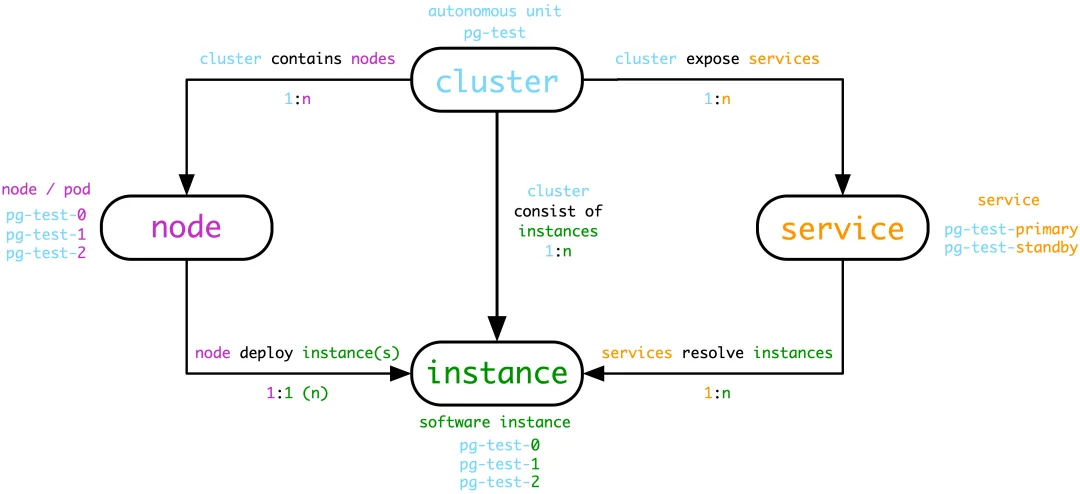
The monitoring model has five levels: cluster, service, instance, database, and node. In this version, service metrics are included in cluster dashboards, and database metrics are included in instance dashboards. The three main views are therefore cluster, instance, and node.

• cls identifies a cluster, for example pg-test-tt.
• ins identifies an instance, for example pg-test-tt-0. It combines the cluster name and an instance number. In this deployment, instance 0 was usually the primary.
• ip identifies a node.

There are also dashboards for the whole fleet, sharded databases, individual databases, connection pools, individual queries, and PgBouncer. I will focus on the main views here.

Features

The system supports routine checks, fault diagnosis, and performance tuning. It includes these dashboards:

• PostgreSQL fleet overview.
• PostgreSQL shard monitoring.
• PostgreSQL cluster monitoring.
• PostgreSQL instance monitoring.
• A dedicated troubleshooting view for a PostgreSQL instance.
• PostgreSQL host monitoring.
• Slow-query analysis.
• Redis fleet overview.
• Redis cluster monitoring.
• Redis instance monitoring.
• PostgreSQL cluster health assessment.

Home and navigation

The home page covers PostgreSQL and Redis. Global metrics appear on the left, cluster navigation on the right, and alerts and events in the middle. Use the navigation links or click a shard, cluster name, instance name, or IP address to open its dashboard.

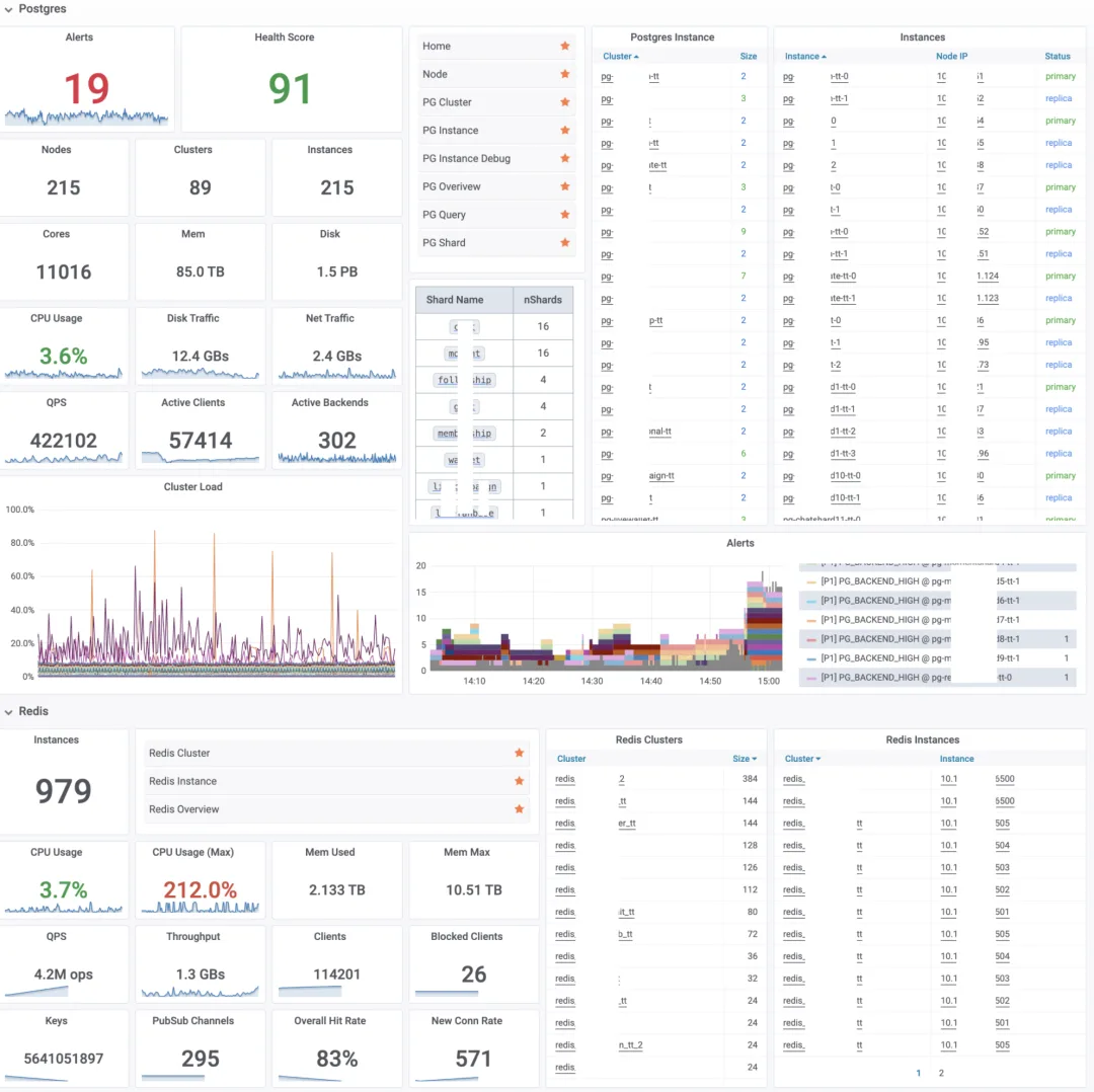
Database metrics

Coverage

At the time, the system exposed about 3,300 metrics per instance, including:

• About 1,000 database and connection-pool metrics, of which 250 were derived through recording rules.
• About 2,000 node metrics, of which 700 were derived through recording rules.

For example, QPS alone produced nearly 30 related metrics:

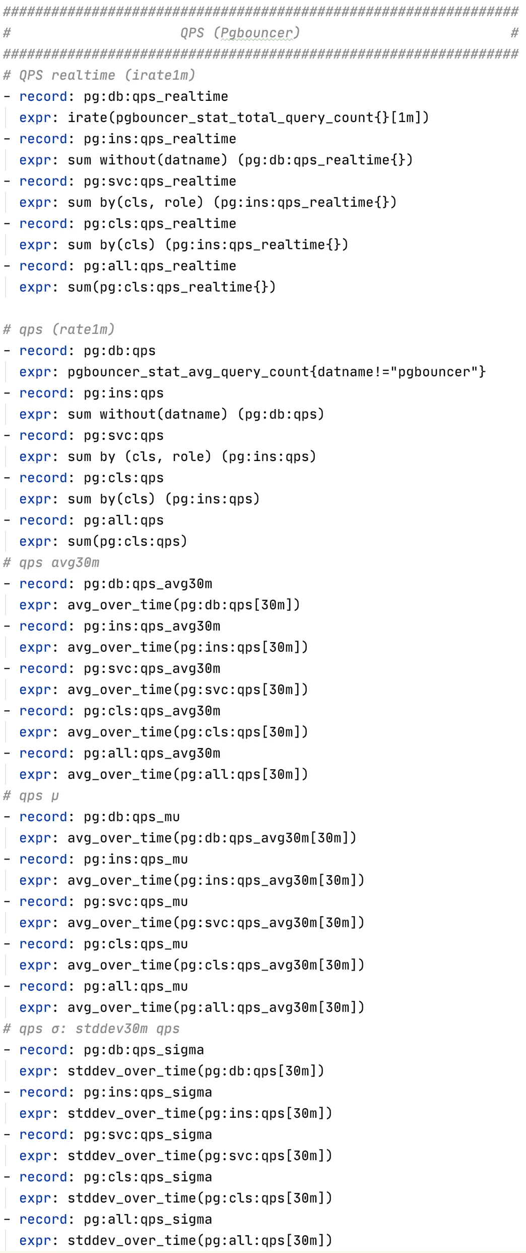
The following sections introduce some of the more useful ones.

The four golden signals

The metrics can be grouped by the four golden signals used in Google SRE practice.

Errors

• Configuration checks: checksums, NUMA, transparent huge pages, synchronous commit, and other important settings.
• Memory and TCP errors, and clock drift.
• Failed hosts, databases, connection pools, or monitoring components.
• Queued clients, idle in transaction sessions, long transactions, deadlocks, broken replication, high rollback counts, and monitoring errors.

Saturation

• PostgreSQL load and node load.
• CPU, memory, disk, and network utilization; cache hit ratios; backend connection use; and connection-pool use.

Traffic

• QPS, TPS, and QPS by statement category.
• Connection-pool traffic, WAL generation, row reads and writes, block access, and buffer access.
• Host disk and network I/O, and memory pages swapped in and out.

Latency

• Average transaction response time, or Xact RT.
• Average query response time, or Query RT.
• Average response time by statement.
• Average disk read and write latency.
• Replication lag in seconds and bytes.
• Monitoring query duration.

PostgreSQL instance monitoring

Instance overview

The overview includes:

• Instance identity: cluster name, ID, host, software version, and other cluster members.
• Important configuration: directories, ports, and configuration file paths.
• Health and role, such as primary or standby.
• Key metrics: PostgreSQL load, replication lag, active backends, queued clients, query latency, TPS, and database age.
• Database load at the current instant and over 1, 5, and 15 minutes.
• Database alerts and events.

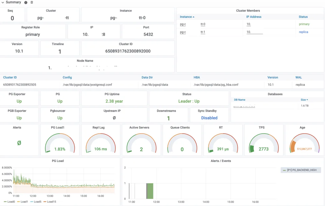
For the definition of PostgreSQL load, see my earlier article, How to Set KPIs for PostgreSQL.

Node overview

The node overview shows:

• CPU, memory, disks, and network interfaces: their capacity, important settings, and core metrics.
• Disk and network-interface details on the right.

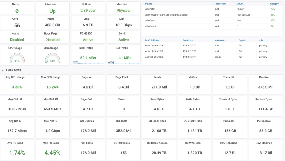
Daily totals

This section summarizes the preceding 24 hours, including query counts and rows returned. The first two rows contain node statistics; the next two mainly contain PostgreSQL statistics.

These totals are useful for usage accounting and capacity assessment.

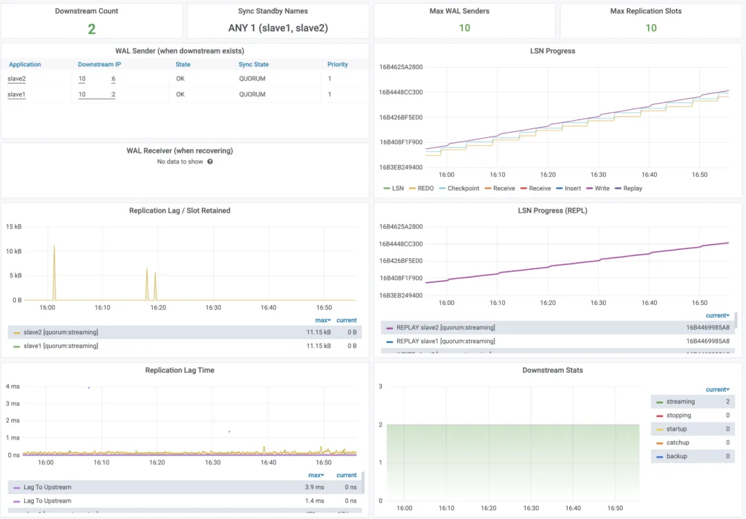
Replication

The replication section shows:

• Replication settings on the current node.
• Lag in seconds and bytes, plus WAL retained by replication slots.
• WAL sender statistics for downstream nodes.
• LSN positions that describe replication progress and durability.
• The number of downstream nodes, which can help detect a lost replication connection.

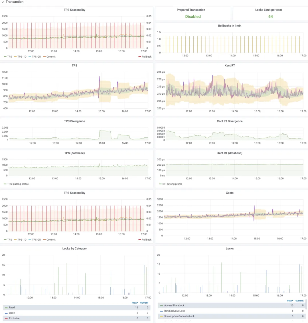
Transactions

The transaction section shows activity through TPS, response time, and locks:

• TPS and comparisons with the preceding two days, plus database transaction and rollback counts.
• Rollback counts and rates.
• Detailed TPS charts. Green bands show ±1 standard deviation and yellow bands show ±3, calculated from the preceding 30 minutes. Values outside the yellow band indicate an unusual change relative to that window.
• Average transaction response time from the connection pool, with the same bands.
• Relative variation of TPS and response time. A dimensionless measure such as (σ/μ)² grows as variation increases relative to the mean.
• TPS and transaction response time by database. Most instances in this deployment had one database, while a few had several.
• Transaction and rollback counts collected directly from PostgreSQL, alongside TPS from the connection pool.
• Lock counts grouped by the eight table-lock modes and by broader read, write, and exclusive categories.

Queries

Query metrics resemble the transaction metrics, but count statements rather than transactions. They help locate slow queries and performance bottlenecks.

• QPS and average query response time, their variation, and comparisons with previous periods.
• This article uses 1 ms as an example warning threshold for average query response time, with closer investigation at 100 ms. Set these thresholds for the workload.

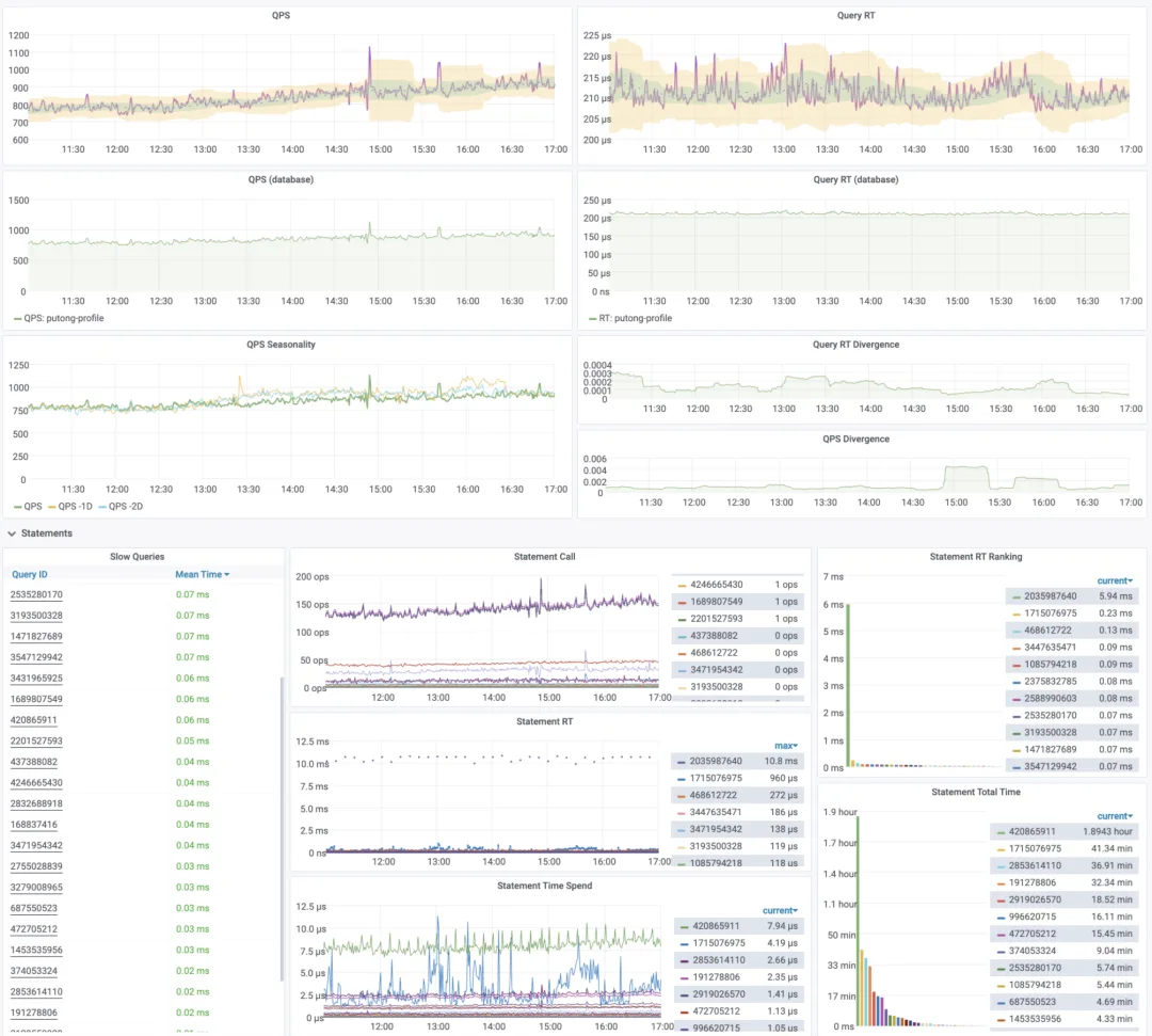
Statements

This section breaks query metrics down by normalized statement. Statements with the same parsed structure after constants are removed belong to the same query class and have a query ID. The slow-query view provides the SQL text and detailed statistics for that ID.

• The list on the left sorts statements by average response time from pg_stat_statements. Click a query ID to open its detailed view.
• The candidates are the 32 queries with the greatest total execution time, excluding monitoring queries and isolated long-running statements with very few calls.
• The right side shows current QPS and average response time for each query, with rankings by response time and total execution time.

Backend processes

Backend metrics describe connections to PostgreSQL. Grouping them in several ways helps diagnose connection surges, slow queries, and waits.

• Counts by backend type, state, database, and wait-event type.
• Active connections, idle in transaction connections, and long transactions.

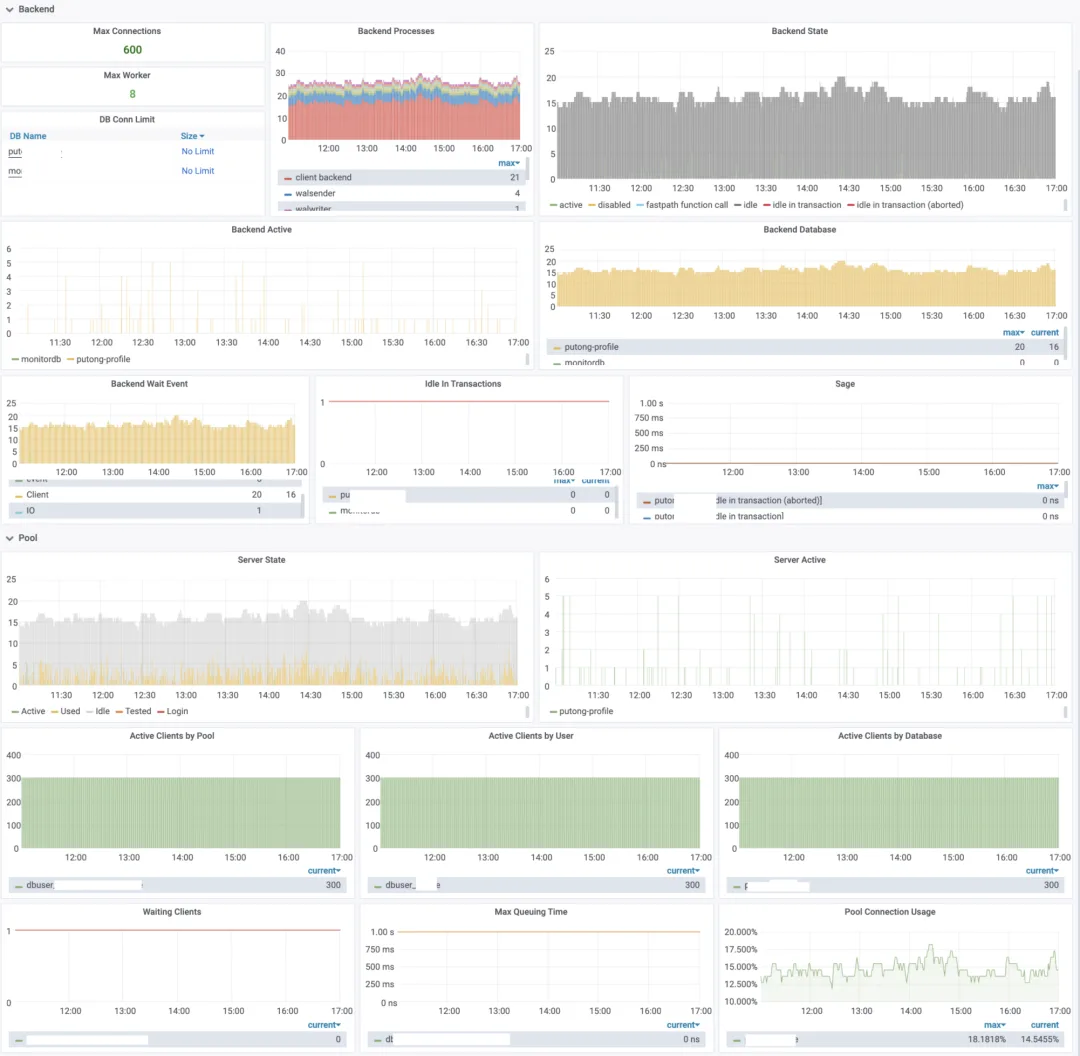
Connection pools

The connection-pool section is similar, but all its metrics come from PgBouncer:

• Server connection states: active, used, idle, tested, and logging in.
• Client connections grouped by user, database, and pool (user:database).
• Waiting clients and the wait time of the client at the head of the queue, which help identify connection backlog.
• The proportion of available pool connections in use.

Database overview

This section draws mainly on pg_stat_database and pg_database, with WAL measurements alongside them:

• WAL generation in bytes per second, an indicator of write activity.
• The shared-buffer hit ratio. A buffer miss can be served by the operating-system page cache or by storage.
• Rows read, inserted, updated, and deleted per second.
• Temporary-file counts and size, which help identify large-query workloads.

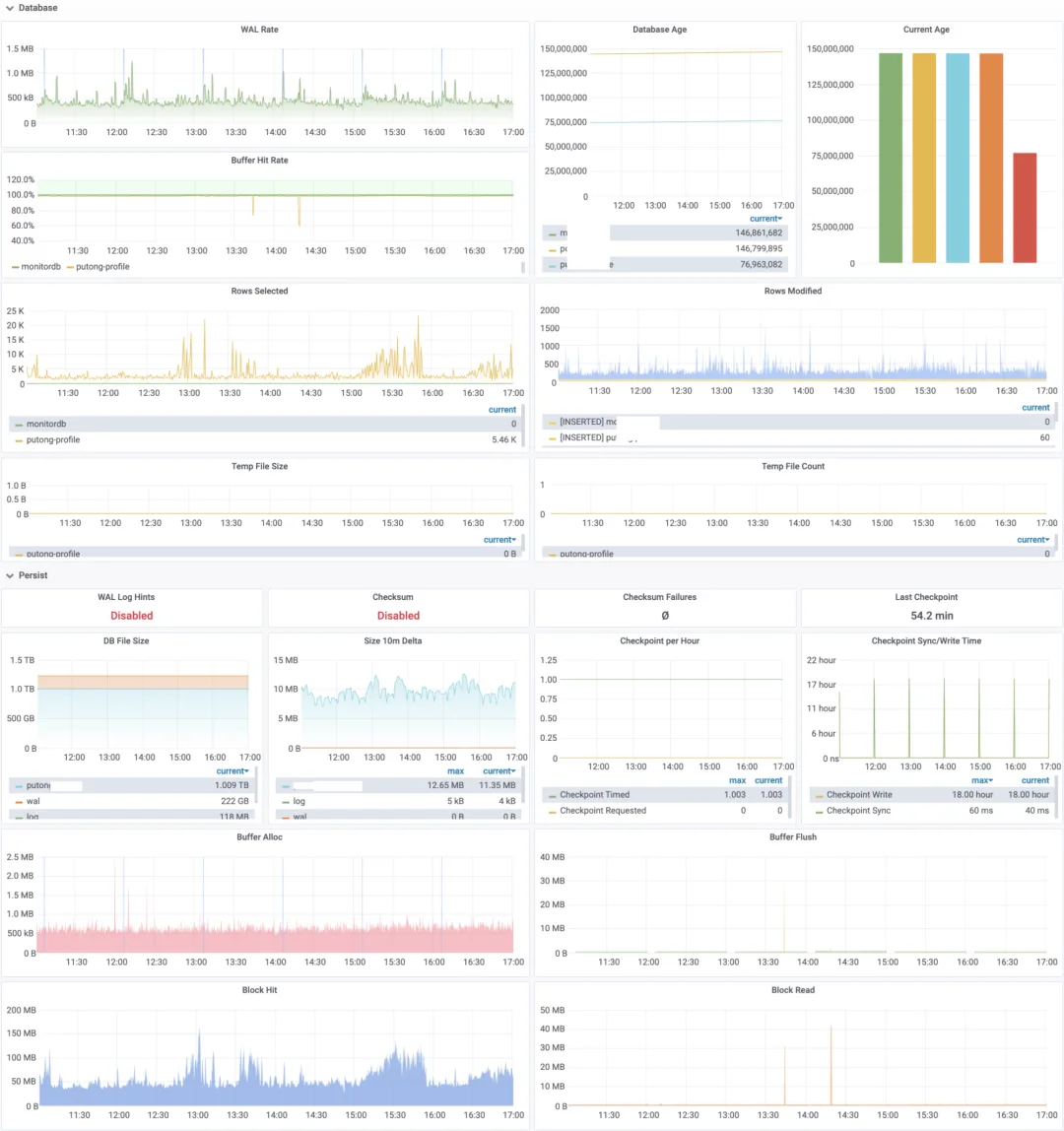
Persistence

Persistence metrics cover writes, checkpoints, and block access:

• Important durability settings and checksum failures, where data checksums are enabled.
• The size and growth of database files, WAL, and logs.
• Checkpoint counts and duration.
• Buffers allocated and written per second, block accesses, and storage reads, also expressed in bytes. The deployment shown here used 8,192-byte PostgreSQL pages and 4,096-byte filesystem blocks.

Exporters

The exporter section monitors the monitoring components themselves:

• Exporter availability, uptime, and scrapes per minute.
• Duration, emitted metric count, and error count for each monitoring query.

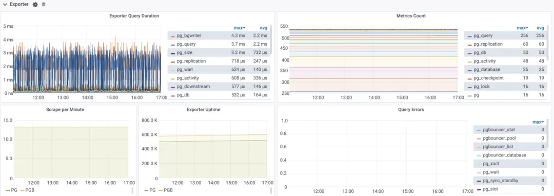
PostgreSQL cluster monitoring

The cluster dashboard is the view I use most often. This deployment serves databases as clusters. Bringing instance and service metrics together makes it easier to check service status.

Most cluster charts extend the instance charts: they compare instances and add cluster- and service-level aggregates.

Cluster overview

The cluster overview adds:

• Timeline and leadership. Failover or switchover changes the primary and advances the timeline.
• Replication topology, including synchronous and asynchronous links.
• Current cluster load and its 1-, 5-, and 15-minute averages, plus each node’s 1-minute load.
• Cluster alerts and events.

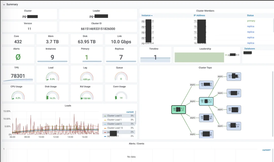
Cluster replication

The cluster dashboard summarizes the replication topology, including:

• The primary and cascading replication nodes, synchronous-commit settings, synchronous standby names, downstream-node counts, and configured standby limits.
• Paired WAL sender and receiver entries for each replication link.
• Replication lag in seconds and bytes, and WAL retained by slots. For example, at a WAL generation rate of 10–100 MB/s, one second of lag corresponds to roughly 10–100 MB of WAL.
• Lag measured from the replica side.
• The number of replicas, useful when a backup or replica initialization changes the expected topology.
• LSN positions across the cluster, showing replication and durability progress.

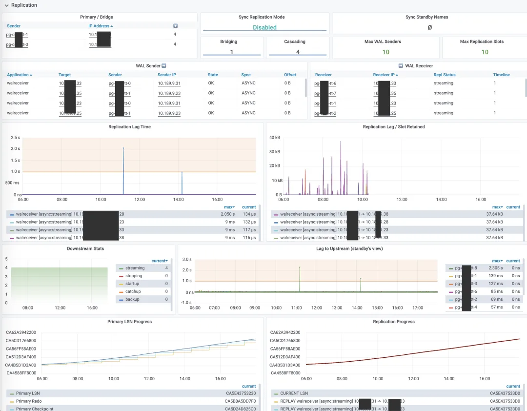
Node metrics

Host metrics are grouped by PostgreSQL cluster.

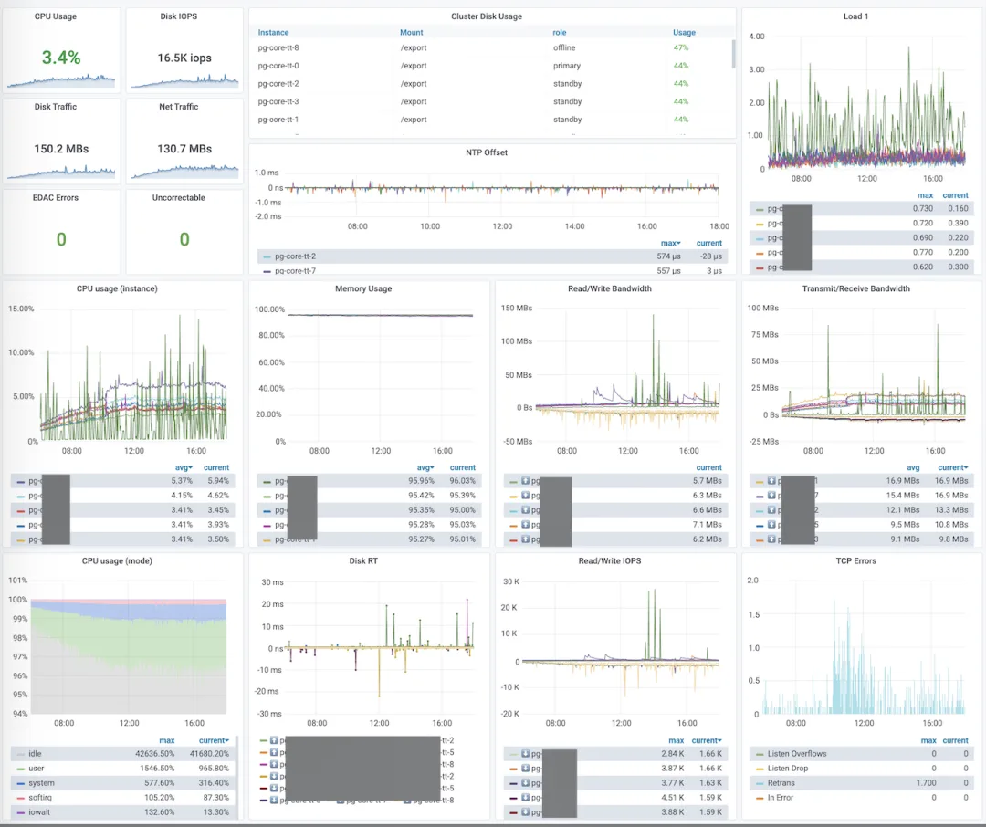
Transactions and queries

These charts resemble the instance views, with additional service-level aggregation. A cluster in this setup usually offered primary and standby services.

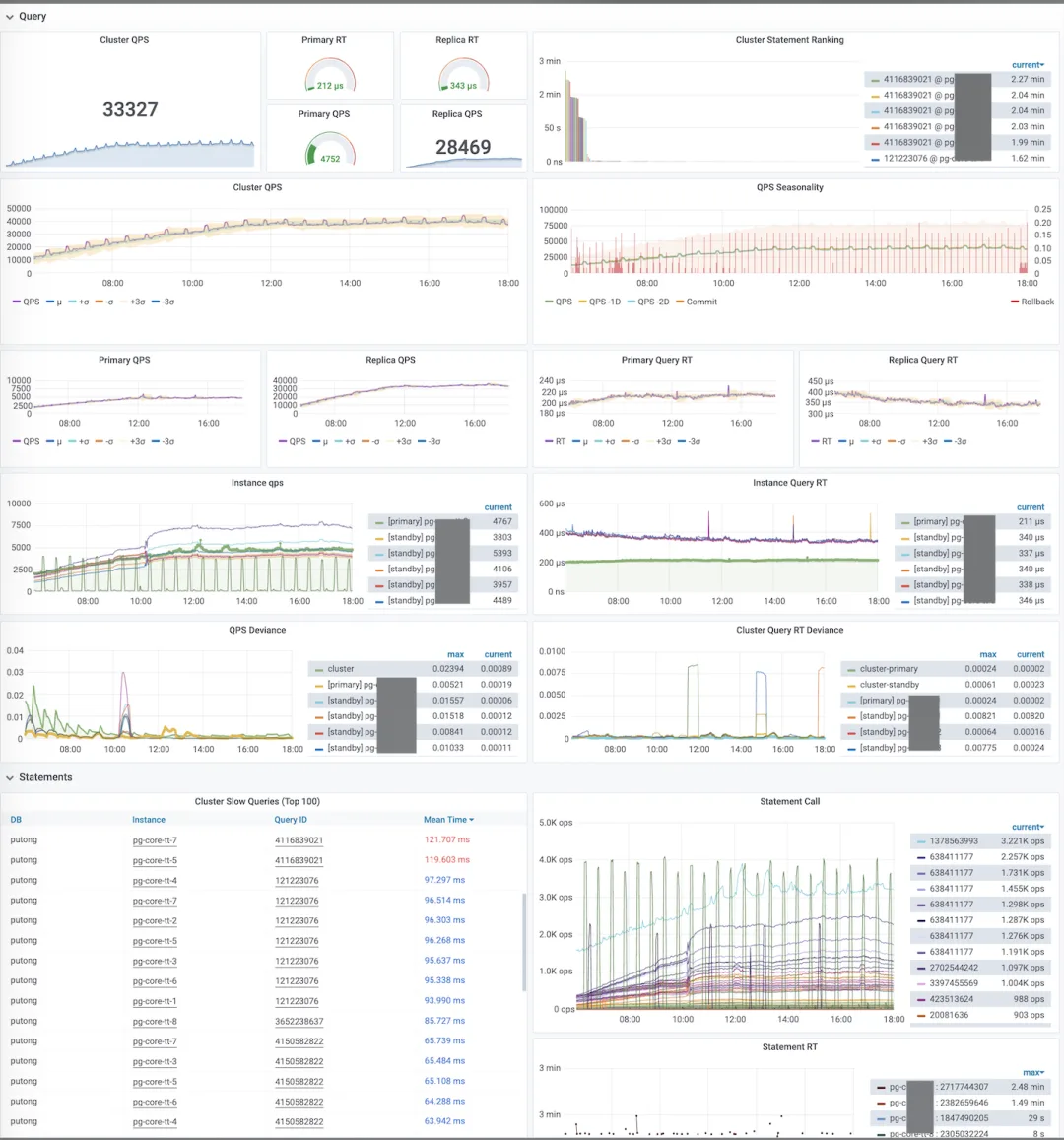
The remaining metrics are similar to those in the instance dashboard.

Slow-query analysis

The slow-query view starts with an overview of queries on the instance. Hover over a query ID to see its SQL, or click it to open Query Detail.

The detailed view has formatted SQL on the left and key metrics on the right:

• Queries per second.
• Current average response time.
• Average rows returned per call.
• Average block I/O time per call.
• Mean, standard deviation, minimum, and maximum response time over the statistics period.
• Calls, rows returned, and execution time in the last day, plus total calls since the statistics were reset.

Charts below show these metrics over the selected time range.

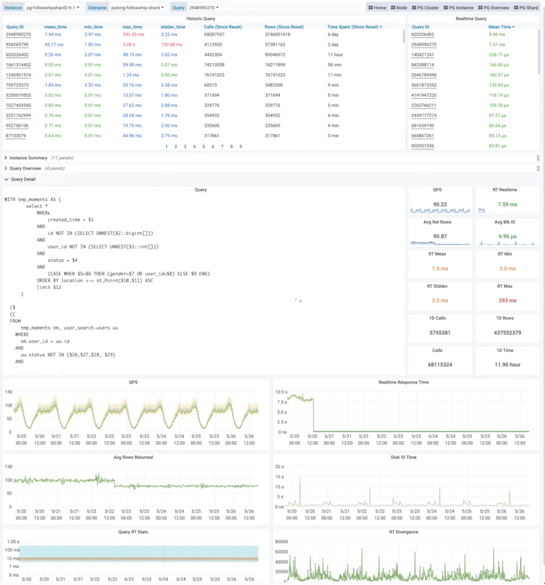
9 - PostgreSQL's KPI

Written in 2020. This article develops a load indicator from PgBouncer transaction time.

PG Load measures accumulated transaction time per second, divided by a chosen concurrency value. It combines the amount of work a database handles with the time that work takes. I use it to track load changes and identify instances that need investigation or a capacity review.

What existing metrics tell us

Database load is usually assessed through several kinds of metrics:

• Traffic: queries per second (QPS) and transactions per second (TPS).
• Latency: query response time (Query RT) and transaction response time (Xact RT).
• Resource use: machine load, CPU utilization, disk I/O, and network I/O.
• Failures and contention: errors and clients waiting for database connections.

Each answers a different question. Errors show failures; a growing connection-pool queue shows contention for connections. Neither alone measures spare capacity. A short queue can coexist with a resource bottleneck, while a long queue can result from a small pool limit.

CPU and I/O metrics show pressure on the host. They help explain database performance when those resources are the bottleneck. But database work can also be limited by locks or occupied connections while CPU utilization remains low. We need a database-level measure to compare with the host metrics.

QPS and TPS count completed work, not its cost. A 10-microsecond query and a 10-second query each count as one call. Throughput is useful when compared with the query mix, latency, and resource use. Load tests can establish a baseline for a known workload.

RT measures service quality. For example, an OLTP service might have a 1 ms response-time target. Rising latency can indicate contention, but does not measure saturation by itself. An average can also hide slow requests; P99 or P99.9 helps show the tail when duration distributions are available.

PG Load combines transaction count and duration into a measure of concurrent work. To derive it, start with two familiar host metrics: load average and CPU utilization.

Deriving PG Load

Linux load average

The first line of top shows load averages for the last 1, 5, and 15 minutes:

$ top -b -n 1
top - 19:27:38 up 18:49,  1 user,  load average: 1.15, 0.72, 0.71

Linux load average counts runnable tasks and tasks in uninterruptible sleep, often waiting for I/O. For CPU-bound work on one core, a load near 1 suggests full CPU demand; values above 1 suggest queuing. On n cores, the corresponding reference is n. Dividing by the number of cores gives a normalized value for comparison.

For CPU-bound work, 0.7 and 1.0 per core can serve as starting points for warning and investigation thresholds. Adjust them to the workload. Because uninterruptible waits also contribute to load, read this value alongside CPU and I/O metrics; it is not a CPU-utilization percentage.

CPU utilization

For one CPU core, utilization can be calculated from its accumulated idle time:

1 - irate(node_cpu_seconds_total{mode="idle"}[1m])

node_cpu_seconds_total{mode="idle"} counts idle seconds. irate uses the last two samples to calculate idle seconds per second. Subtracting that fraction from 1 gives the fraction of time the core was busy. For a multi-core CPU, average the utilization of its cores.

This suggests a similar measure for a PostgreSQL backend: the fraction of time it is active. Load average also suggests how to extend that measure to multiple backends: add their active time and normalize by concurrency.

From backend time to database load

Start with a one-second window and normalize by the number of available backends:

The third example raises a choice: count only query execution, or count the whole transaction, including time between statements. We will use transaction time and explain that choice below. Client time waiting for a backend is separate and is not included.

For a longer window or more backends, the calculation is the same:

pg_load = pg_active_seconds / time_period / parallel

• pg_active_seconds is the sum of active seconds across the observed backends during the window.
• time_period is the window duration in seconds.
• parallel is the concurrency value used for normalization.

A value of 0 means no observed activity. A value of 100% means one second of active time per second per unit of chosen concurrency. It does not, by itself, establish a capacity limit.

If active seconds are available as a cumulative counter, use its rate of increase:

rate(pg_active_seconds[time_period]) / parallel

The remaining choices are how to measure active time and which concurrency value to use.

Calculating PG Load

Count query time or transaction time?

For a single query in an autocommit transaction, query time and transaction time are close. For a transaction with several statements, they can differ substantially. In the example above, 0.6 seconds of query execution plus 0.2 seconds idle in transaction gives 60% by query time and 80% by transaction time.

Query time measures execution. Transaction time measures how long the transaction occupies its backend. An idle transaction may use little CPU, but it still occupies a connection and can retain locks or snapshots. I use transaction time here to include that occupancy in the load measure.

Obtain accumulated transaction time

pg_stat_activity shows the current state of PostgreSQL backends. Repeated samples can estimate how many backends are active over time, but the view itself is a snapshot, not an accumulated duration counter.

PgBouncer provides the counters needed for this calculation. Its SHOW STATS command reports statistics for each database, including:

• total_xact_count: completed transactions.
• total_query_count: executed queries.
• total_xact_time: accumulated transaction time.
• total_query_time: accumulated query time.

The raw time counters use microseconds. The exported pgbouncer_stat_total_xact_time series used below is already in seconds. See PgBouncer statistics.

Apply rate to that counter to obtain transaction seconds per second over 1, 5, or 15 minutes. For the most recent interval, irate uses the last two samples. Then sum across databases with sum without (datname) to obtain an instance-level value:

- record: pg:ins:xact_time_realtime
  expr: sum without (datname) (irate(pgbouncer_stat_total_xact_time{}[1m]))
- record: pg:ins:xact_time_rate1m
  expr: sum without (datname) (rate(pgbouncer_stat_total_xact_time{}[1m]))
- record: pg:ins:xact_time_rate5m
  expr: sum without (datname) (rate(pgbouncer_stat_total_xact_time{}[5m]))
- record: pg:ins:xact_time_rate15m
  expr: sum without (datname) (rate(pgbouncer_stat_total_xact_time{}[15m]))

The result estimates concurrent transaction work. One continuously occupied backend contributes one transaction second per second; 64 contribute 64. This lets us compare periods on the same instance, but comparison across instance sizes needs a normalization factor.

Normalize by CPU count

This method uses CPU count as the concurrency reference. It is useful for CPU-bound work, but is not a measured limit on PostgreSQL concurrency. Connection limits, parallel workers, lock waits, and I/O also affect how much work an instance can sustain.

On a 64-core host, 64 backends continuously occupied by transactions produce a load of 64 / 64 = 100%. With 128 such backends, the result is 128 / 64 = 200%.

Divide the transaction-time rates by CPU count to obtain the PG Load series:

- record: pg:ins:load0
  expr:  pg:ins:xact_time_realtime / on (ip) group_left()  node:ins:cpu_count
- record: pg:ins:load1
  expr: pg:ins:xact_time_rate1m  / on (ip) group_left()  node:ins:cpu_count
- record: pg:ins:load5
  expr: pg:ins:xact_time_rate5m  / on (ip) group_left()  node:ins:cpu_count
- record: pg:ins:load15
  expr: pg:ins:xact_time_rate15m  / on (ip) group_left()  node:ins:cpu_count

The relationship with throughput and latency

Active seconds per second can also be approximated by TPS × average transaction RT, or QPS × average query RT. Use the same observation window and express RT in seconds. For example, 1,000 queries per second at 1 ms each accumulate 1000 × 0.001 = 1 query second per second.

With transaction time and CPU normalization, this gives:

tps * xact_rt / cpu_count

TPS alone ignores the cost of each transaction; RT alone ignores how many transactions run. Their product accounts for both. The recording rules above obtain that accumulated work directly from the time counter.

Using PG Load

Alerting: slow queries occupy the connection pool

In the production incident below, an application change introduced a slow query. Slow queries occupied the connection pool, and requests accumulated. Both PG Load and RT rose clearly; the drop in TPS was less conspicuous. After this incident, we added PG Load1 and PG Load0 to our alerting rules.

The example thresholds are 50% for a warning and 70% for an alert. Choose thresholds from the workload baseline and response-time target. A value of 500% means accumulated transaction time is five times the CPU-normalized reference; latency, queue length, and wait metrics help locate the cause.

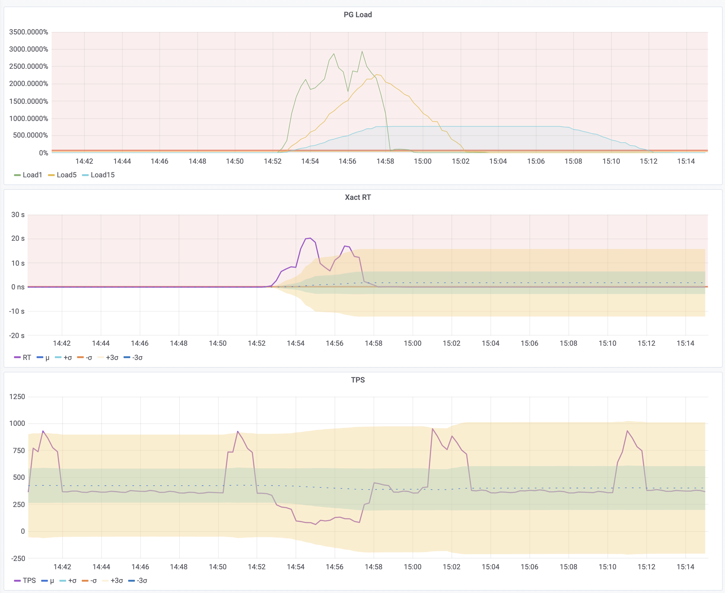
Capacity assessment

For capacity planning, compare 15-minute PG Load averages and peaks with the cluster’s historical baseline, response-time targets, and expected growth. This helps identify clusters that need more detailed review of capacity, query cost, or resource limits.

Compare PG Load with CPU utilization as well. The transaction counter excludes CPU time spent directly on unrelated host work. Backups and maintenance can still increase transaction duration through resource contention, so their effect can appear in PG Load.

Sustained load of 30%–50% can be a starting point for a capacity review. Whether to expand capacity depends on peak demand and the headroom needed for that workload.

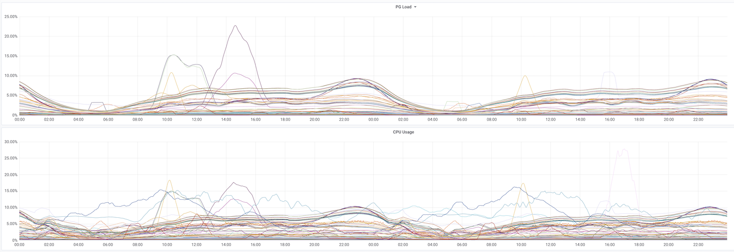
10 - An Overview of PostgreSQL Monitoring

This article describes a monitoring system from December 2018. Its dashboard layout and statistics-collector details belong to that period.

Using monitoring to manage PostgreSQL

Managing PostgreSQL requires an understanding of its operating state. Monitoring brings this information together for routine checks, fault diagnosis, and performance tuning. I planned a series of articles about the design, implementation, and use of this monitoring system.

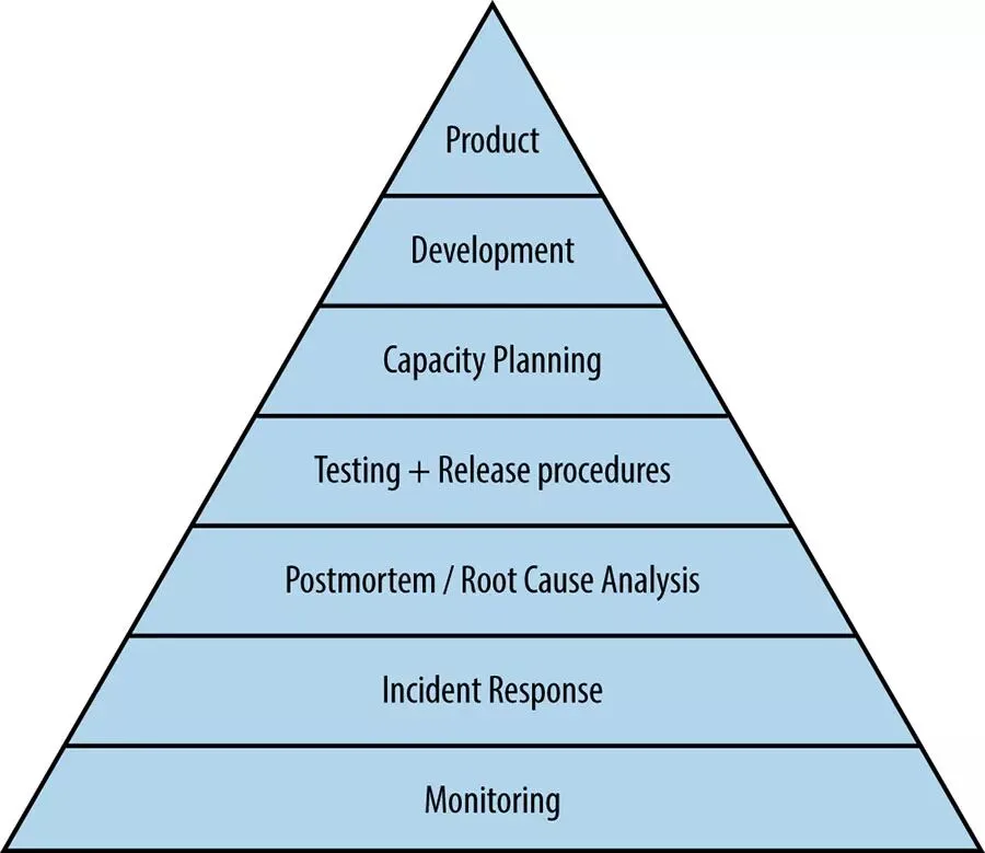
The PostgreSQL dashboard

These are the dashboards I used in a working environment. The most frequently used view monitored one database instance. It had seven main sections: overview, operating system, database activity and sessions, replication, checkpoints and WAL, conflicts, and database object statistics.

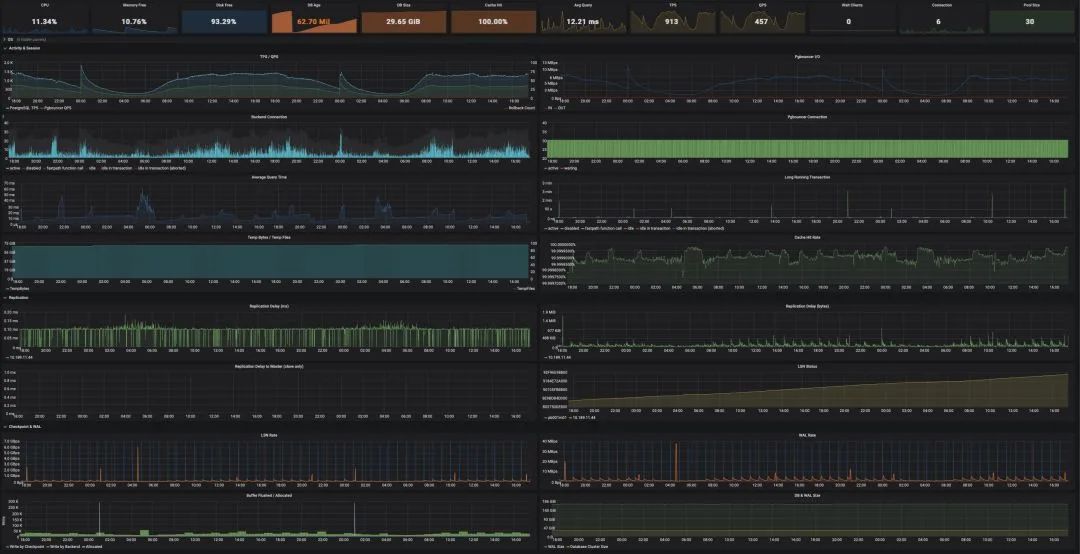
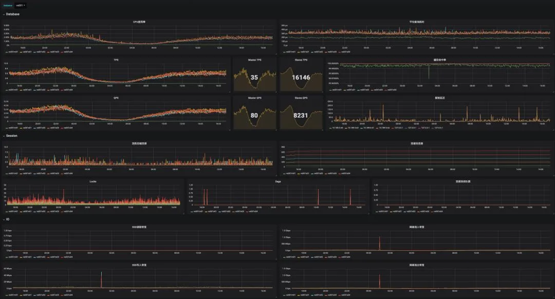
System architecture

This system uses Prometheus, Grafana, Consul, and exporters.

Exporters read metrics from databases, connection pools, and hosts. Prometheus discovers exporters through Consul and scrapes their metrics. Grafana displays the data, while Alertmanager handles alerts.

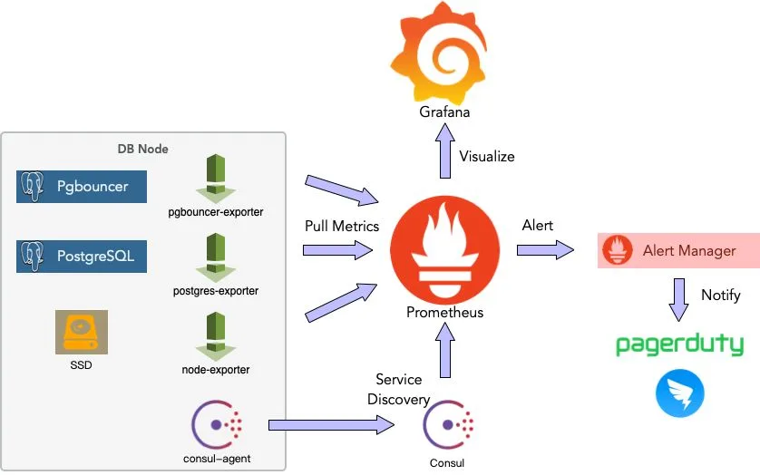
Monitoring metrics

For each metric, identify the question it answers, its data source, and the meaning of changes in its value. This helps interpret charts and guides command-line investigation. The following sections describe the main metrics in the single-instance dashboard.

Overview

The overview contains key metrics that help narrow down a problem at a glance:

• CPU utilization, average query time, TPS, QPS, queued pool clients, and active connections indicate load.
• Free memory helps identify pressure that can lead to processes being killed.
• Free disk space shows whether storage is close to full.
• Database age indicates proximity to transaction ID wraparound limits.
• Database size and cache hit ratio help identify changes in activity.

Operating system

The operating-system section includes:

• CPU utilization and system load.
• Memory usage, including changes in the operating-system cache.
• Network and disk throughput, and disk IOPS.

Compare these metrics with database activity to identify resource pressure and investigate possible hardware faults.

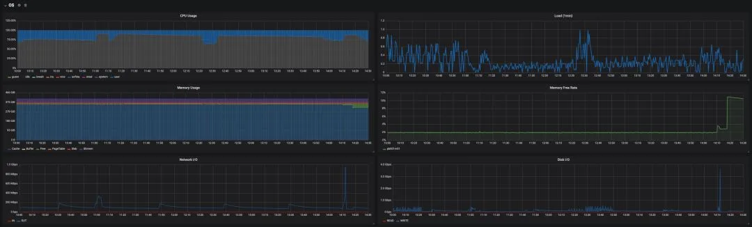
Database activity and sessions

Activity and session metrics show the database’s current workload:

• TPS, QPS, and average response time describe traffic and latency.
• The cache hit ratio here refers to PostgreSQL’s shared buffers. It excludes the operating-system file cache.
• Connection counts by state show how sessions are being used. Active connections show work in progress; inspect idle in transaction sessions to find why their transactions remain open.
• Complex or large queries can create temporary files. Heavy temporary-file I/O can reduce performance.

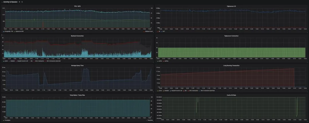
Replication

Replication lag helps assess replica freshness and investigate replication faults.

The primary reports how far replicas lag in bytes of WAL and, from PostgreSQL 10, replication lag times. A replica can also report the time since its last replayed transaction, although this is not an exact measure of current lag: it can increase while an idle primary produces no new transactions.

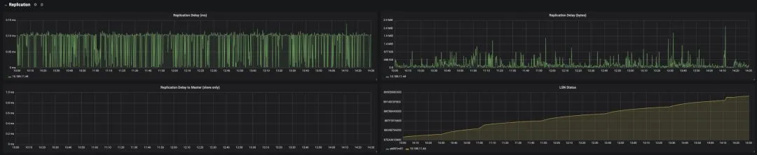
Checkpoints and WAL

Checkpoints consume I/O by writing dirty pages. With full_page_writes enabled, the first change to a page after a checkpoint also writes a full-page image to WAL. This can increase disk and network traffic and contribute to performance problems.

Useful metrics include:

• WAL generation rate.
• LSN growth rate.
• Buffers written by checkpoints and by backends. Heavy backend writes can indicate that checkpoint or background-writing settings need review.
• Database and WAL size.

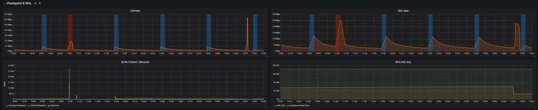
Locks and conflicts

Counts by lock type help explain database activity and investigate lock conflicts.

Object statistics

Object-level statistics help locate the source of a problem:

• Index and sequential scan counts per table. For frequent sequential scans on large tables, use query plans to check whether the indexes suit the workload.
• Tuple reads and writes, table size, and table age.
• The proportion of dead tuples, which indicates vacuum demand and can help investigate bloat. It is not the same as the physical bloat ratio; statistics-based bloat estimates provide another view.
• Function call counts and execution time.

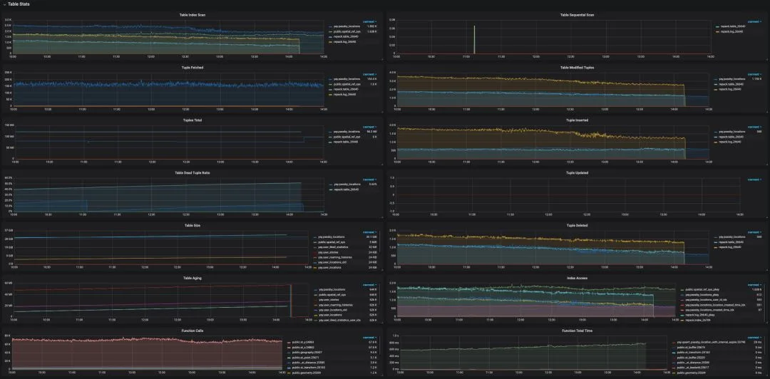
Metric sources

The statistics collector

In the PostgreSQL versions discussed here, many metrics came from the built-in statistics collector. System views expose the data through SQL; the PostgreSQL documentation defines each view. Some common views are listed below.

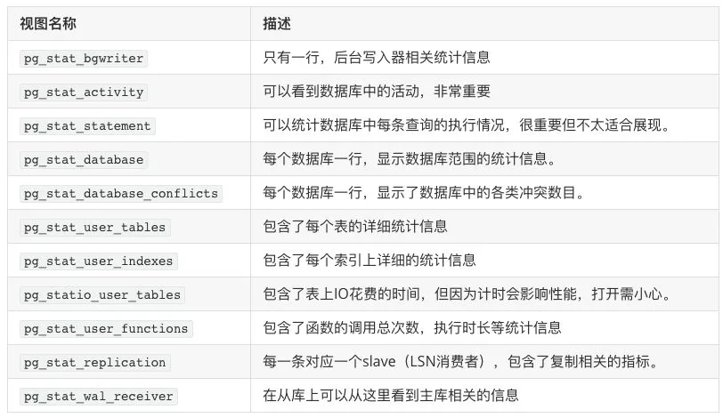
The PostgreSQL 11 statistics documentation describes several details to account for:

• Cumulative statistics were not updated continuously. Backends reported their counts before becoming idle, so work still in progress was not yet fully reflected in those totals.
• Statistics reports were normally spaced at least 500 ms apart (PGSTAT_STAT_INTERVAL). Current activity, controlled by track_activities, followed a separate mechanism.
• Repeated statistics queries within one transaction could reuse the same snapshot. pg_stat_clear_snapshot() cleared it so the next query could fetch a new one.
• The required track_* settings had to be enabled in postgresql.conf.

These details describe the older collector process. PostgreSQL 15 replaced it with shared-memory cumulative statistics; use the documentation for your server version when interpreting update and snapshot behavior.

Catalogs and other system views

Other catalogs and views provide useful data too. For example, pg_database supplies database metadata used to assess transaction ID age, and pg_locks shows locks and waits. Built-in functions provide further measurements, including database size.

Further articles

This article introduces the architecture and main metrics. Later articles cover implementation details and how to use the metrics to investigate problems.

11 - Relation Bloat Monitoring and Management

This article was written in 2018. It explains statistics-based bloat estimates and maintenance practices from that period.

PostgreSQL uses MVCC to let transactions work with different row versions. Old versions can leave tables and indexes larger than their live data requires. Routine vacuum makes space reusable; a rewrite can return excess space to the filesystem. This article explains how to measure bloat and choose when to reorganize a relation.

Relation Bloat Overview

If a relation occupies 100 GB and a compact copy would occupy 60 GB, its estimated bloat rate is (100 - 60) / 100 = 40%.

Regular VACUUM reclaims dead-tuple space for reuse within the table. It can also truncate empty pages at the end of the file. It does not compact live rows across the whole table, so free space between live pages usually remains allocated.

VACUUM FULL copies live tuples to a new file to compact the table. It holds an AccessExclusiveLock for the operation, blocking reads and writes. pg_repack allows most reads and writes to continue, but needs brief exclusive locks during setup and the final swap.

Measure bloat before choosing which relations to rewrite. Set the threshold and schedule from workload, available disk space, and maintenance windows.

Measuring Relation Bloat

Estimate the bloat rate with 1 - compact_size / actual_size. The compact size includes live tuples and necessary page, tuple, and alignment overhead.

Relation size is available from PostgreSQL. The next step is to measure or estimate the space that live tuples need.

Measuring Tuple and Free Space

pgstattuple scans a relation and reports live tuples, dead tuples, and free space. tuple_percent uses a 0–100 scale. Thus 1 - tuple_percent / 100 is the share outside live tuples, including necessary storage overhead. The sample calls this value bloat, but it is not the exact fraction a rewrite can reclaim.

vonng@[local]:5432/bench# select *,
                          1.0 - tuple_len::numeric / table_len as bloat
                          from pgstattuple('pgbench_accounts');
┌─[ RECORD 1 ]───────┬────────────────────────┐
│ table_len          │ 136642560              │
│ tuple_count        │ 1000000                │
│ tuple_len          │ 121000000              │
│ tuple_percent      │ 88.55                  │
│ dead_tuple_count   │ 16418                  │
│ dead_tuple_len     │ 1986578                │
│ dead_tuple_percent │ 1.45                   │
│ free_space         │ 1674768                │
│ free_percent       │ 1.23                   │
│ bloat              │ 0.11447794889088729017 │
└────────────────────┴────────────────────────┘

See the PostgreSQL 10 pgstattuple reference for field definitions and the pgstatindex function for B-tree indexes.

Two other supplied extensions help inspect relation storage:

• pg_freespacemap reports recorded free space in each page.
• pageinspect reads the contents of individual pages.

For routine monitoring, an estimate is usually enough to identify relations for closer inspection. Measuring every live tuple requires a full relation scan, which can add substantial I/O when repeated across many tables.

PostgreSQL 9.5 added pgstattuple_approx to the pgstattuple extension. It estimates some values to reduce the amount of data scanned. Its cost depends on how much of the relation must be read.

Use statistics-based estimates for frequent monitoring across many tables. Scan selected relations when you need a more precise measurement.

Estimating Bloat Rate

The estimate uses three values from table and column statistics:

• Average tuple width avgwidth: calculated from column-level statistical data, used to estimate space occupied in compact state
• Tuple count: pg_class.reltuples: used to estimate space occupied in compact state
• Page count: pg_class.relpages: used to measure actually used space

The estimate is:

1 - (reltuples * avgwidth) / (block_size - pageheader) / relpages

Here block_size is page size, default 8192, pageheader is header overhead, default 24 bytes. Page size minus header size gives actual space available for tuple storage. Therefore, (reltuples * avgwidth) gives estimated total tuple size, and dividing by the former gives expected pages needed to compactly store all tuples. Finally, expected page count divided by actual page count gives utilization rate, and 1 minus utilization rate gives bloat rate.

Difficulties

Estimating average tuple length requires accounting for:

• When tuples contain null values, headers will have null bitmaps
• There’s padding between headers and data sections, requiring boundary alignment consideration
• Some field types also have alignment requirements

Calculating Average Tuple Length

The diagram shows the PostgreSQL tuple layout used to estimate average tuple length.

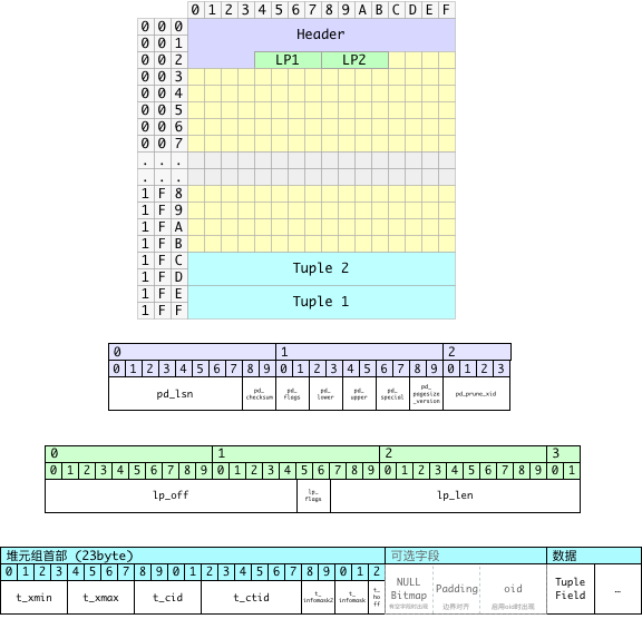
Space occupied by a tuple can be divided into three parts:

• Fixed-length line pointer (4 bytes, strictly speaking this isn’t part of the tuple, but it corresponds one-to-one with tuples)
• Variable-length header
  • Fixed-length part 23 bytes
  • When tuples contain null values, a null bitmap appears, with each field occupying one bit, so its length is the number of fields divided by 8, rounded up
  • After the null bitmap, padding is needed to MAXALIGN, usually 8
  • If the table has the WITH OIDS option enabled, tuples also have a 4-byte OID, but we don’t consider this case here
• Data section

Therefore, a tuple’s average length (including corresponding line pointer) can be calculated as:

avg_size_tuple = 4 + avg_size_hdr + avg_size_data

The key is finding average header length and average data section length.

Calculating Average Header Length

The main variables in average header length are null bitmap and padding alignment. To estimate average tuple header length, we need several parameters:

• Average header length without null bitmap (with padding): normhdr
• Average header length with null bitmap (with padding): nullhdr
• Proportion of tuples with null values: nullfrac

Estimate average header length with:

avg_size_hdr =  nullhdr * nullfrac + normhdr * (1 - nullfrac)

Since headers without null bitmaps are 23 bytes long, aligned to 8-byte boundaries gives 24 bytes, the above formula becomes:

avg_size_hdr =  nullhdr * nullfrac +  24 * (1 - nullfrac)

To round a length up to an 8-byte boundary, use:

padding = lambda x: ((x + 7) >> 3) << 3

Calculating Average Data Section Length

Average data section length mainly depends on each field’s average width and null rate, plus trailing alignment.

The following SQL can calculate average tuple data section width for all tables using statistical information:

SELECT schemaname, tablename, sum((1 - null_frac) * avg_width)
FROM pg_stats GROUP BY (schemaname, tablename);

For example, this SQL can get average tuple length for table app.apple from the pg_stats system statistics view:

SELECT
  count(*),                        -- number of fields
  ceil(count(*) / 8.0),            -- bytes occupied by null bitmap
  max(null_frac),                  -- maximum null rate
  sum((1 - null_frac) * avg_width) -- average width of data section
FROM pg_stats
where schemaname = 'app' and tablename = 'apple';

-[ RECORD 1 ]-----------
count | 47
ceil  | 6
max   | 1
sum   | 1733.76873471724

max(null_frac) is an approximation for the fraction of rows with any NULL. Column statistics do not describe how NULL values overlap across columns.

Integration

The function below combines those estimates. It assumes 8-byte alignment and uses the server’s block size. It returns NULL when statistics are unavailable. It estimates heap space only; TOAST, fillfactor, and column alignment can affect the result.

CREATE OR REPLACE FUNCTION public.pg_table_bloat(relation regclass)
RETURNS double precision
LANGUAGE plpgsql
AS $function$
DECLARE
  _schemaname text;
  _tablename  text;
  tuples      double precision;
  pages       integer;
  nullheader  double precision;
  nullfrac    double precision;
  datawidth   double precision;
  avgtuplelen double precision;
  blocksize   integer := current_setting('block_size')::integer;
BEGIN
  SELECT n.nspname, c.relname, c.reltuples, c.relpages
    INTO _schemaname, _tablename, tuples, pages
    FROM pg_class c JOIN pg_namespace n ON n.oid = c.relnamespace
    WHERE c.oid = relation;

  IF pages = 0 THEN RETURN 0; END IF;
  IF pages IS NULL OR tuples < 0 THEN RETURN NULL; END IF;

  SELECT 23 + ceil(count(*) / 8.0),
         max(null_frac),
         sum((1 - null_frac) * avg_width)
    INTO nullheader, nullfrac, datawidth
    FROM pg_stats
    WHERE schemaname = _schemaname AND tablename = _tablename
      AND NOT inherited;

  IF datawidth IS NULL THEN RETURN NULL; END IF;

  avgtuplelen := 4 + ceil(datawidth / 8.0) * 8
    + (1 - nullfrac) * 24 + nullfrac * ceil(nullheader / 8.0) * 8;

  RETURN greatest(0, 1 - ceil(tuples * avgtuplelen / (blocksize - 24)) / pages);
END;
$function$;

Batch Calculation

For database-wide monitoring, a view can estimate many relations from catalog statistics. This separate example estimates B-tree index bloat:

CREATE SCHEMA IF NOT EXISTS monitor;
CREATE OR REPLACE VIEW monitor.pg_bloat_indexes AS
  WITH btree_index_atts AS (
      SELECT
        pg_namespace.nspname,
        indexclass.relname                                                          AS index_name,
        indexclass.reltuples,
        indexclass.relpages,
        pg_index.indrelid,
        pg_index.indexrelid,
        indexclass.relam,
        tableclass.relname                                                          AS tablename,
        generate_series(1, pg_index.indnatts)                                        AS attnum,
        pg_index.indexrelid                                                         AS index_oid
      FROM ((((pg_index
        JOIN pg_class indexclass ON ((pg_index.indexrelid = indexclass.oid)))
        JOIN pg_class tableclass ON ((pg_index.indrelid = tableclass.oid)))
        JOIN pg_namespace ON ((pg_namespace.oid = indexclass.relnamespace)))
        JOIN pg_am ON ((indexclass.relam = pg_am.oid)))
      WHERE ((pg_am.amname = 'btree' :: NAME) AND (indexclass.relpages > 0))
  ), index_item_sizes AS (
      SELECT
        ind_atts.nspname,
        ind_atts.index_name,
        ind_atts.reltuples,
        ind_atts.relpages,
        ind_atts.relam,
        ind_atts.indrelid                                    AS table_oid,
        ind_atts.index_oid,
        (current_setting('block_size' :: TEXT)) :: NUMERIC   AS bs,
        8                                                    AS maxalign,
        24                                                   AS pagehdr,
        CASE
        WHEN (max(COALESCE(pg_stats.null_frac, (0) :: REAL)) = (0) :: FLOAT)
          THEN 2
        ELSE 6
        END                                                  AS index_tuple_hdr,
        sum((((1) :: FLOAT - COALESCE(pg_stats.null_frac, (0) :: REAL)) *
             (COALESCE(pg_stats.avg_width, 1024)) :: FLOAT)) AS nulldatawidth
      FROM ((pg_attribute
        JOIN btree_index_atts ind_atts
          ON (((pg_attribute.attrelid = ind_atts.indexrelid) AND (pg_attribute.attnum = ind_atts.attnum))))
        JOIN pg_stats ON (((pg_stats.schemaname = ind_atts.nspname) AND (((pg_stats.tablename = ind_atts.tablename) AND
                                                                          ((pg_stats.attname) :: TEXT =
                                                                           pg_get_indexdef(pg_attribute.attrelid,
                                                                                           (pg_attribute.attnum) :: INTEGER,
                                                                                           TRUE))) OR
                                                                         ((pg_stats.tablename = ind_atts.index_name) AND
                                                                          (pg_stats.attname = pg_attribute.attname))))))
      WHERE (pg_attribute.attnum > 0)
      GROUP BY ind_atts.nspname, ind_atts.index_name, ind_atts.reltuples, ind_atts.relpages, ind_atts.relam,
        ind_atts.indrelid, ind_atts.index_oid, (current_setting('block_size' :: TEXT)) :: NUMERIC, 8 :: INTEGER
  ), index_aligned_est AS (
      SELECT
        index_item_sizes.maxalign,
        index_item_sizes.bs,
        index_item_sizes.nspname,
        index_item_sizes.index_name,
        index_item_sizes.reltuples,
        index_item_sizes.relpages,
        index_item_sizes.relam,
        index_item_sizes.table_oid,
        index_item_sizes.index_oid,
        COALESCE(ceil((((index_item_sizes.reltuples * ((((((((6 + index_item_sizes.maxalign) -
                                                             CASE
                                                             WHEN ((index_item_sizes.index_tuple_hdr %
                                                                    index_item_sizes.maxalign) = 0)
                                                               THEN index_item_sizes.maxalign
                                                             ELSE (index_item_sizes.index_tuple_hdr %
                                                                   index_item_sizes.maxalign)
                                                             END)) :: FLOAT + index_item_sizes.nulldatawidth)
                                                          + (index_item_sizes.maxalign) :: FLOAT) - (
                                                           CASE
                                                           WHEN (((index_item_sizes.nulldatawidth) :: INTEGER %
                                                                  index_item_sizes.maxalign) = 0)
                                                             THEN index_item_sizes.maxalign
                                                           ELSE ((index_item_sizes.nulldatawidth) :: INTEGER %
                                                                 index_item_sizes.maxalign)
                                                           END) :: FLOAT)) :: NUMERIC) :: FLOAT) /
                        ((index_item_sizes.bs - (index_item_sizes.pagehdr) :: NUMERIC)) :: FLOAT) +
                       (1) :: FLOAT)), (0) :: FLOAT) AS expected
      FROM index_item_sizes
  ), raw_bloat AS (
      SELECT
        current_database()                                                           AS dbname,
        index_aligned_est.nspname,
        pg_class.relname                                                             AS table_name,
        index_aligned_est.index_name,
        (index_aligned_est.bs * ((index_aligned_est.relpages) :: BIGINT) :: NUMERIC) AS totalbytes,
        index_aligned_est.expected,
        CASE
        WHEN ((index_aligned_est.relpages) :: FLOAT <= index_aligned_est.expected)
          THEN (0) :: NUMERIC
        ELSE (index_aligned_est.bs *
              ((((index_aligned_est.relpages) :: FLOAT - index_aligned_est.expected)) :: BIGINT) :: NUMERIC)
        END                                                                          AS wastedbytes,
        CASE
        WHEN ((index_aligned_est.relpages) :: FLOAT <= index_aligned_est.expected)
          THEN (0) :: NUMERIC
        ELSE (((index_aligned_est.bs * ((((index_aligned_est.relpages) :: FLOAT -
                                          index_aligned_est.expected)) :: BIGINT) :: NUMERIC) * (100) :: NUMERIC) /
              (index_aligned_est.bs * ((index_aligned_est.relpages) :: BIGINT) :: NUMERIC))
        END                                                                          AS realbloat,
        pg_relation_size((index_aligned_est.table_oid) :: REGCLASS)                  AS table_bytes,
        stat.idx_scan                                                                AS index_scans
      FROM ((index_aligned_est
        JOIN pg_class ON ((pg_class.oid = index_aligned_est.table_oid)))
        JOIN pg_stat_user_indexes stat ON ((index_aligned_est.index_oid = stat.indexrelid)))
  ), format_bloat AS (
      SELECT
        raw_bloat.dbname                                             AS database_name,
        raw_bloat.nspname                                            AS schema_name,
        raw_bloat.table_name,
        raw_bloat.index_name,
        round(
            raw_bloat.realbloat)                                     AS bloat_pct,
        round((raw_bloat.wastedbytes / (((1024) :: FLOAT ^
                                         (2) :: FLOAT)) :: NUMERIC)) AS bloat_mb,
        round((raw_bloat.totalbytes / (((1024) :: FLOAT ^ (2) :: FLOAT)) :: NUMERIC),
              3)                                                     AS index_mb,
        round(
            ((raw_bloat.table_bytes) :: NUMERIC / (((1024) :: FLOAT ^ (2) :: FLOAT)) :: NUMERIC),
            3)                                                       AS table_mb,
        raw_bloat.index_scans
      FROM raw_bloat
  )
  SELECT
    format_bloat.database_name                    as datname,
    format_bloat.schema_name                      as nspname,
    format_bloat.table_name                       as relname,
    format_bloat.index_name                       as idxname,
    format_bloat.index_scans                      as idx_scans,
    format_bloat.bloat_pct                        as bloat_pct,
    format_bloat.table_mb,
    format_bloat.index_mb - format_bloat.bloat_mb as actual_mb,
    format_bloat.bloat_mb,
    format_bloat.index_mb                         as total_mb
  FROM format_bloat
  ORDER BY format_bloat.bloat_mb DESC;

COMMENT ON VIEW monitor.pg_bloat_indexes IS 'index bloat monitor';

In the original 3 TB database, this view took about 50 ms. It reads catalog statistics rather than scanning every index page. Catalog access and relation-size lookups still have a cost, and stale or incomplete statistics affect the estimate. The result is a screening tool for candidate indexes.

Handling Table Bloat

Use VACUUM FULL when a maintenance window allows exclusive table access. For online reorganization, pg_repack reduces the duration of exclusive locking.

• pg_repack documentation

The original PostgreSQL 10 environment used the PGDG package below. Select the package built for your PostgreSQL major version:

yum install pg_repack10

Using pg_repack

pg_repack uses the usual PostgreSQL client connection parameters.

Before using pg_repack, you need to create the pg_repack extension in the database to be reorganized:

CREATE EXTENSION pg_repack;

Example commands:

# Repack mydb; use 5 workers for index builds and wait up to 10 seconds for locks
pg_repack -d mydb -j 5 -T 10 --no-kill-backend

# Repack one table; skip it if conflicting locks remain after 10 seconds
pg_repack mydb -t public.mytable -T 10 --no-kill-backend

# Clean specific index myschema.myindex, must use full name with schema
pg_repack mydb -i myschema.myindex --no-kill-backend

-T controls lock waiting, not total runtime. Without --no-kill-backend, pg_repack can cancel and later terminate conflicting sessions. A full-table repack needs a primary key or a suitable unique index on NOT NULL columns. See the option reference.

pg_repack Strategy

Schedule pg_repack during low-traffic periods. It consumes CPU, disk I/O, and extra storage, and can increase query latency and replication lag.

For example, select candidate tables during a low-traffic period. The following view supplies the columns used by the scheduling example; total_mb measures current disk usage in MiB, including indexes and TOAST:

CREATE OR REPLACE VIEW monitor.pg_bloat_tables AS
SELECT current_database() AS datname,
       n.nspname,
       c.relname,
       pg_total_relation_size(c.oid) / 1048576.0 AS total_mb,
       b.ratio * 100 AS bloat_pct
FROM pg_class c
JOIN pg_namespace n ON n.oid = c.relnamespace
CROSS JOIN LATERAL (SELECT public.pg_table_bloat(c.oid) AS ratio) b
WHERE c.relkind = 'r'
  AND n.nspname NOT IN ('pg_catalog', 'information_schema')
  AND n.nspname NOT LIKE 'pg_toast%';

The shell functions return one table name per line and accept table names as separate quoted arguments:

repack_tables() {
    local db=$1 relname old_size new_size
    shift
    for relname in "$@"; do
        old_size=$(psql -X -d "$db" -v ON_ERROR_STOP=1 -v relation="$relname" -At <<'SQL'
SELECT pg_size_pretty(pg_total_relation_size(:'relation'::regclass));
SQL
) || return
        printf 'Repack %s: %s before\n' "$relname" "$old_size"
        pg_repack --dbname="$db" --table="$relname" --wait-timeout=10 --no-kill-backend || return
        new_size=$(psql -X -d "$db" -v ON_ERROR_STOP=1 -v relation="$relname" -At <<'SQL'
SELECT pg_size_pretty(pg_total_relation_size(:'relation'::regclass));
SQL
) || return
        printf 'Repack %s: %s -> %s\n' "$relname" "$old_size" "$new_size"
    done
}

get_bloat_tables() {
    psql -X -d "$1" -v ON_ERROR_STOP=1 -At <<'SQL'
WITH bloat_tables AS (
    SELECT format('%I.%I', nspname, relname) AS relname,
           total_mb, bloat_pct
    FROM monitor.pg_bloat_tables
    WHERE nspname NOT IN ('dba', 'monitor', 'trash')
)
(SELECT relname FROM bloat_tables
 WHERE total_mb < 256 AND bloat_pct > 40
 ORDER BY bloat_pct DESC LIMIT 64)
UNION
(SELECT relname FROM bloat_tables
 WHERE total_mb >= 256 AND total_mb < 1024 AND bloat_pct > 30
 ORDER BY bloat_pct DESC LIMIT 16)
UNION
(SELECT relname FROM bloat_tables
 WHERE total_mb >= 1024 AND total_mb <= 4096 AND bloat_pct > 20
 ORDER BY bloat_pct DESC LIMIT 4);
SQL
}

These size thresholds use current disk usage, including the table, indexes, and TOAST:

• From small tables < 256 MiB with bloat rate > 40%, select TOP64
• From medium tables 256 MiB to 1 GiB with bloat rate > 30%, select TOP16
• From large tables 1 GiB to 4 GiB with bloat rate > 20%, select TOP4

This example reorganizes selected tables during the early-morning low-traffic period and handles tables whose total disk usage exceeds 4 GiB manually. Adjust the schedule to your workload.

pg_repack Principles

pg_repack builds a compact copy and records concurrent changes with a trigger. After replaying those changes, it swaps storage through the system catalogs. Index-only repacks build a replacement index concurrently, then swap and drop the old index.

Reorganizing Tables

1. Create an empty table with the same schema as the original table but without indexes
2. Create a log table corresponding to the original table to record changes that occur on that table during pg_repack operation
3. Add a row trigger to the original table to record all INSERT, DELETE, UPDATE operations in the corresponding log table
4. Copy data from the old table to the new empty table
5. Create the same indexes on the new table
6. Apply incremental changes from the log table to the new table
7. Swap table, index, and TOAST storage through the system catalogs
8. Drop the old storage

Reorganizing Indexes

1. Use CREATE INDEX CONCURRENTLY to create a new index on the original table, maintaining the same definition as the old index
2. Swap the old and new indexes in the system catalogs
3. Delete the old index

pg_repack Operating Checks

• Schedule around long transactions and conflicting maintenance. Inspect lock waits before deciding whether to cancel a session.
• Budget disk for the replacement table, indexes, and change log. The project recommends free space of about twice the table-and-index size for a full repack.
• Monitor WAL volume, replica replay lag, and free disk space throughout the copy and index build. WAL is generated during the operation, not just at the final swap.
• After interruption, inspect the installed version’s cleanup guidance and the remaining objects before retrying. Temporary-object names and cleanup behavior vary by version.

See the pg_repack requirements and implementation notes when planning the operation.

12 - Monitoring Table Size in PostgreSQL

This 2018 article explains physical storage for ordinary PostgreSQL tables.

Table Storage Layout

An ordinary table has its own storage and may also have a TOAST table:

• Main table: stores row data, relkind='r'.
• TOAST table: stores out-of-line values when needed, relkind='t'. Some tables have no TOAST table.

A table and each of its indexes are separate relations:

• Main relation: stores tuples.
• Index relation: stores index tuples.

Each relation may have four forks:

• main: the relation’s main file, numbered 0

• fsm: stores information about free space in the main fork, numbered 1

• vm: stores information about visibility in the main fork, numbered 2

• init: used for unlogged tables and indexes, numbered 3

Each fork is stored in one or more files. The default segment size is 1 GiB; it can be changed when PostgreSQL is built.

To account for a table’s storage, include these relations:

• Main table’s main relation (single)
• Main table’s indexes (multiple)
• TOAST table’s main relation (single)
• TOAST table’s index (single)

Include every fork that exists for each relation: main, fsm, vm, and init. The init fork applies to unlogged relations.

Getting Table’s Associated Relations

The following query lists relation OIDs. Forks share a relation OID; they do not have independent OIDs. The left join keeps tables that have no TOAST table:

select
  nsp.nspname,
  rel.relname,
  rel.relnamespace    as nspid,
  rel.oid             as relid,
  rel.reltoastrelid   as toastid,
  toastind.indexrelid as toastindexid,
  ind.indexes
from
  pg_namespace nsp
  join pg_class rel on nsp.oid = rel.relnamespace
  CROSS JOIN LATERAL (select array_agg(indexrelid) as indexes from pg_index where indrelid = rel.oid) ind
  LEFT JOIN LATERAL (select indexrelid from pg_index where indrelid = rel.reltoastrelid) toastind ON true
where nspname not in ('pg_catalog', 'information_schema') and rel.relkind = 'r';

 nspname |  relname   |  nspid  |  relid  | toastid | toastindexid |      indexes
---------+------------+---------+---------+---------+--------------+--------------------
 public  | aoi        | 4310872 | 4320271 | 4320274 |      4320276 | {4325606,4325605}
 public  | poi        | 4310872 | 4332324 | 4332327 |      4332329 | {4368886}

Statistical Functions

PostgreSQL provides size functions for each part:

For routine monitoring, group storage into table and index space. For ordinary tables, pg_table_size plus pg_indexes_size equals pg_total_relation_size.

The following identities describe the components; they are formulas, not a complete SQL query:

 pg_table_size(relid)
     = pg_relation_size(relid, 'main')
     + pg_relation_size(relid, 'fsm')
     + pg_relation_size(relid, 'vm')
     + pg_relation_size(relid, 'init')
     + COALESCE(pg_total_relation_size(reltoastrelid), 0)

 pg_indexes_size(relid)
     = (SELECT COALESCE(sum(pg_total_relation_size(indexrelid)), 0)
        FROM pg_index WHERE indrelid = relid)

A TOAST table has one index. Use pg_total_relation_size(reltoastrelid) to include both the TOAST table and its index.

Example: Table and Related Relation Sizes

SELECT
  oid,
  relname,
  relnamespace::RegNamespace::Text               as nspname,
  relkind                                        as relkind,
  reltuples                                      as tuples,
  relpages                                       as pages,
  pg_total_relation_size(oid)                    as size
  FROM pg_class
WHERE oid = ANY(array(SELECT 16418 as id -- main
UNION ALL SELECT indexrelid FROM pg_index WHERE indrelid = 16418 -- index
UNION ALL SELECT reltoastrelid FROM pg_class WHERE oid = 16418)); -- toast

Wrap the query in a table-returning function for reuse. Replace the example OID with a table in your database:

CREATE OR REPLACE FUNCTION pg_table_size_detail(relation RegClass)
  RETURNS TABLE(
    id      oid,
    pid     oid,
    relname name,
    nspname text,
    relkind "char",
    tuples  bigint,
    pages   integer,
    size    bigint
  )
AS $$
BEGIN
  RETURN QUERY
  SELECT
    rel.oid,
    relation::oid,
    rel.relname,
    rel.relnamespace :: RegNamespace :: Text as nspname,
    rel.relkind                              as relkind,
    rel.reltuples::bigint                    as tuples,
    rel.relpages                             as pages,
    pg_total_relation_size(rel.oid)          AS size
  FROM pg_class rel
  WHERE rel.oid = ANY (array(
      SELECT relation::oid AS id -- main
      UNION ALL SELECT indexrelid FROM pg_index WHERE indrelid = relation -- index
      UNION ALL SELECT reltoastrelid FROM pg_class WHERE oid = relation)); -- toast
END;
$$
LANGUAGE PlPgSQL;

SELECT * FROM pg_table_size_detail(16418);

Each row’s size includes that relation’s attached storage. The main table row already includes its indexes and TOAST, so do not sum this column. tuples and pages come from planner statistics and can lag behind current data.

Sample result from the original environment:

geo=# select * from  pg_table_size_detail(4325625);
   id    |   pid   |        relname        | nspname  | relkind |  tuples  |  pages  |    size
---------+---------+-----------------------+----------+---------+----------+---------+-------------
 4325628 | 4325625 | pg_toast_4325625      | pg_toast | t       |   154336 |   23012 |   192077824
 4419940 | 4325625 | idx_poi_adcode_btree  | gaode    | i       | 62685464 |  172058 |  1409499136
 4419941 | 4325625 | idx_poi_cate_id_btree | gaode    | i       | 62685464 |  172318 |  1411629056
 4419942 | 4325625 | idx_poi_lat_btree     | gaode    | i       | 62685464 |  172058 |  1409499136
 4419943 | 4325625 | idx_poi_lon_btree     | gaode    | i       | 62685464 |  172058 |  1409499136
 4419944 | 4325625 | idx_poi_name_btree    | gaode    | i       | 62685464 |  335624 |  2749431808
 4325625 | 4325625 | gaode_poi             | gaode    | r       | 62685464 | 2441923 | 33714962432
 4420005 | 4325625 | idx_poi_position_gist | gaode    | i       | 62685464 |  453374 |  3714039808
 4420044 | 4325625 | poi_position_geohash6 | gaode    | i       | 62685464 |  172058 |  1409499136

Example: Relation Size Details Summary

select
  nsp.nspname,
  rel.relname,
  rel.relnamespace    as nspid,
  rel.oid             as relid,
  rel.reltoastrelid   as toastid,
  toastind.indexrelid as toastindexid,
  pg_total_relation_size(rel.oid)  as size,
  pg_relation_size(rel.oid) + pg_relation_size(rel.oid,'fsm')
  + pg_relation_size(rel.oid,'vm')
  + pg_relation_size(rel.oid,'init') AS relsize,
  pg_indexes_size(rel.oid)         as indexsize,
  COALESCE(pg_total_relation_size(reltoastrelid), 0) AS toastsize,
  ind.indexids,
  ind.indexnames,
  ind.indexsizes
from pg_namespace nsp
  join pg_class rel on nsp.oid = rel.relnamespace
  LEFT JOIN LATERAL (select indexrelid from pg_index where indrelid = rel.reltoastrelid) toastind ON true
  CROSS JOIN LATERAL (select array_agg(indexrelid ORDER BY indexrelid) AS indexids,
                      array_agg(indexrelid::regclass ORDER BY indexrelid) AS indexnames,
                      array_agg(pg_total_relation_size(indexrelid) ORDER BY indexrelid) AS indexsizes
              from pg_index where indrelid = rel.oid) ind
where nspname not in ('pg_catalog', 'information_schema') and rel.relkind = 'r';

13 - PostgreSQL Server Log Configuration

This article was written in 2018. The table definitions below use the 23-column PostgreSQL 10 CSV format, and the Filebeat example uses the legacy prospectors configuration.

CSV logs can be imported into PostgreSQL tables or queried through file_fdw for analysis.

Log Configuration

log_destination = 'csvlog'
logging_collector = on
log_directory = 'log'
log_filename = 'postgresql-%a.log'
log_min_duration_statement = 1000
log_checkpoints = on
log_lock_waits = on
log_statement = 'ddl'
log_replication_commands = on
log_timezone = 'UTC'
log_autovacuum_min_duration = 1000

track_io_timing = on
track_functions = all
track_activity_query_size = 16384

The last three settings collect runtime statistics; they do not control log output. logging_collector and track_activity_query_size require a server restart. The weekday filename repeats each week. Configure rotation and retention to match how long you need to keep the files.

Log Collection

The original setup used Filebeat to forward local files to Kafka. Replace the paths and broker address with your own. This legacy example starts at the end of existing files and joins lines by a timestamp pattern, with a 20-line limit. It does not provide general CSV record framing for arbitrary multiline messages.

filebeat.prospectors:
  - type: log
    enabled: true
    paths:
      - /pg/data/log/postgresql-*.csv
    document_type: db-trace
    tail_files: true
    multiline.pattern: '^20\d\d-\d\d-\d\d'
    multiline.negate: true
    multiline.match: after
    multiline.max_lines: 20

max_cpus: 1

filebeat.config.modules:
  path: ${path.config}/modules.d/*.yml
  reload.enabled: false

queue.mem:
  events: 1024
  flush.min_events: 0
  flush.timeout: 1s

output.kafka:
  hosts: ["kafka.example.com:9092"]
  topics:
    - topic: 'log.db'

CSV Log Format

PostgreSQL can query its logs as rows. The following table matches the PostgreSQL 10 CSV fields. Later server versions add columns; use the table definition for the server that wrote the log:

-- Log table structure
create table postgresql_log
(
  log_time               timestamp(3) with time zone,
  user_name              text,
  database_name          text,
  process_id             integer,
  connection_from        text,
  session_id             text   not null,
  session_line_num       bigint not null,
  command_tag            text,
  session_start_time     timestamp with time zone,
  virtual_transaction_id text,
  transaction_id         bigint,
  error_severity         text,
  sql_state_code         text,
  message                text,
  detail                 text,
  hint                   text,
  internal_query         text,
  internal_query_pos     integer,
  context                text,
  query                  text,
  query_pos              integer,
  location               text,
  application_name       text,
  PRIMARY KEY (session_id, session_line_num)
);

Importing Logs

Import a closed CSV log file with COPY. The server must be able to read the file. For a file on the client machine, use psql’s \copy. Import complete files after rotation, and import each file only once.

COPY postgresql_log FROM '/pg/data/log/postgresql-Mon.csv' WITH (FORMAT csv);

Mapping Logs

Use file_fdw to query local CSV files without copying them into a table. Run the setup with the required extension and server-file privileges. The example assumes English weekday names and existing files under /pg/data/log; adjust the paths to match the log output. Query an individual child table if some weekday files do not yet exist.

CREATE SCHEMA IF NOT EXISTS monitor;

-- This session only
SET search_path = monitor, pg_catalog;

-- extension
CREATE EXTENSION IF NOT EXISTS file_fdw WITH SCHEMA monitor;

-- log parent table: empty
CREATE TABLE monitor.pg_log
(
  log_time               timestamp(3) with time zone,
  user_name              text,
  database_name          text,
  process_id             integer,
  connection_from        text,
  session_id             text,
  session_line_num       bigint,
  command_tag            text,
  session_start_time     timestamp with time zone,
  virtual_transaction_id text,
  transaction_id         bigint,
  error_severity         text,
  sql_state_code         text,
  message                text,
  detail                 text,
  hint                   text,
  internal_query         text,
  internal_query_pos     integer,
  context                text,
  query                  text,
  query_pos              integer,
  location               text,
  application_name       text,
  PRIMARY KEY (session_id, session_line_num)
);
COMMENT ON TABLE monitor.pg_log IS 'PostgreSQL csv log schema';
-- local file server
CREATE SERVER IF NOT EXISTS pg_log FOREIGN DATA WRAPPER file_fdw;
-- Change filename to actual path
CREATE FOREIGN TABLE IF NOT EXISTS monitor.pg_log_mon() INHERITS (monitor.pg_log) SERVER pg_log OPTIONS (filename '/pg/data/log/postgresql-Mon.csv', format 'csv');
CREATE FOREIGN TABLE IF NOT EXISTS monitor.pg_log_tue() INHERITS (monitor.pg_log) SERVER pg_log OPTIONS (filename '/pg/data/log/postgresql-Tue.csv', format 'csv');
CREATE FOREIGN TABLE IF NOT EXISTS monitor.pg_log_wed() INHERITS (monitor.pg_log) SERVER pg_log OPTIONS (filename '/pg/data/log/postgresql-Wed.csv', format 'csv');
CREATE FOREIGN TABLE IF NOT EXISTS monitor.pg_log_thu() INHERITS (monitor.pg_log) SERVER pg_log OPTIONS (filename '/pg/data/log/postgresql-Thu.csv', format 'csv');
CREATE FOREIGN TABLE IF NOT EXISTS monitor.pg_log_fri() INHERITS (monitor.pg_log) SERVER pg_log OPTIONS (filename '/pg/data/log/postgresql-Fri.csv', format 'csv');
CREATE FOREIGN TABLE IF NOT EXISTS monitor.pg_log_sat() INHERITS (monitor.pg_log) SERVER pg_log OPTIONS (filename '/pg/data/log/postgresql-Sat.csv', format 'csv');
CREATE FOREIGN TABLE IF NOT EXISTS monitor.pg_log_sun() INHERITS (monitor.pg_log) SERVER pg_log OPTIONS (filename '/pg/data/log/postgresql-Sun.csv', format 'csv');